Learning Center

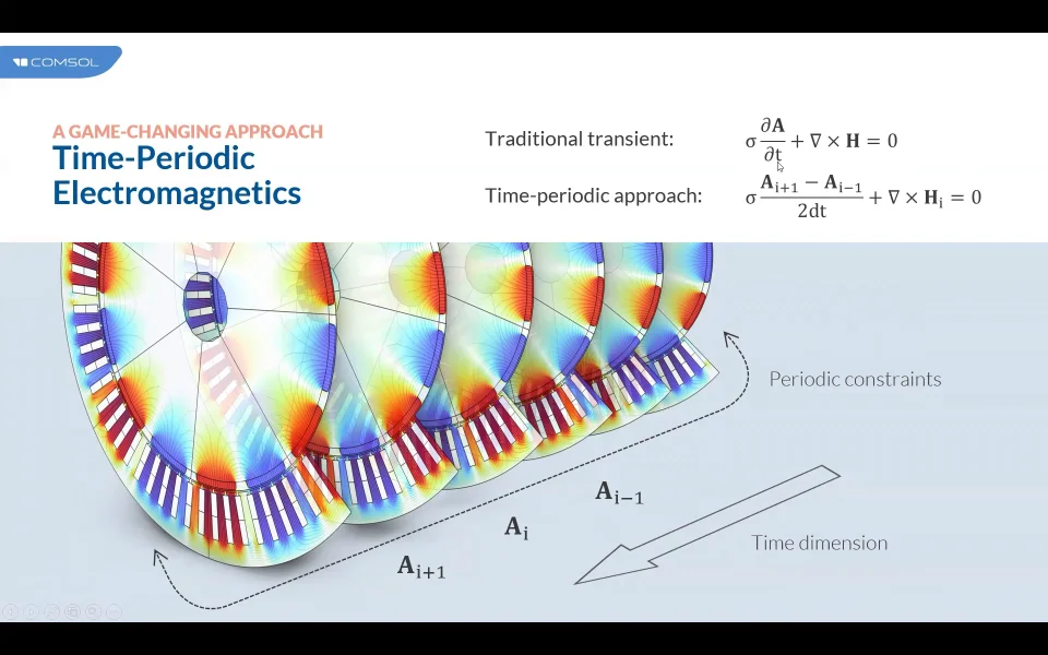
The Time-Periodic Motor Modeling approach in COMSOL Multiphysics offers an alternative to the traditional transient method for simulating electric motors. In the traditional transient approach, the magnetic vector potential is solved using its time derivative, meaning each solution depends only on previous solutions—the method only "knows about the past." This approach is versatile and can answer nearly any question about a system, including losses and time-dependent torque. However, in an electric motor, the solution is periodic: the result at phase zero should equal the result at phase 2π. The time-periodic approach exploits this by rewriting the differential equation with the time variable represented implicitly as a phase in an extra dimension. Unlike the frequency domain study, which is only valid for linear materials through linearization, the time-periodic approach supports nonlinear materials and problems. It solves for the true B-H curve and captures genuine transient behavior, making it especially suitable for parametric studies such as efficiency maps and temperature maps, as well as optimization. The dedicated interface is accessed through the ACDC branch under Rotating Machinery, Magnetic, Time Periodic. Key settings include electrical frequency and the number of time frames, which define the phase-step resolution analogous to time steps. The interface automatically handles rotational periodicity and continuity by detecting the number of sectors and poles, and it automatically computes torque and includes loss models—such as the Steinmetz model for laminated cores and resistive losses for windings—directly within the boundary conditions, eliminating the need for separate loss calculation features. The problem is solved as a single stationary study, with rotating domains added by right-clicking the interface. Results are evaluated as functions of phase rather than explicit time, allowing plots of quantities at specific phase angles as well as cycle-averaged quantities like losses and torque, which closely match those from the transient approach. The principal advantage of the time-periodic approach emerges in multiphysics coupling. In the traditional workflow, calculating electromagnetic heating requires running a magnetic transient simulation, performing an FFT for losses, running a heat transfer simulation, and then iterating between the two until convergence. With the time-periodic approach, the electromagnetic and heat transfer physics are solved together in one stationary study, reaching equilibrium without iteration. Because a stationary study is used, previous solutions can serve as initial conditions for subsequent ones, greatly accelerating parametric sweeps such as efficiency maps that vary speed and applied current. Since the time-dependent solution is written in an extra dimension, the frequency response is computed inherently, which benefits coupling to structural mechanics and acoustics—for example, generating Campbell diagrams that show sound pressure levels across shaft speeds and harmonics. The approach also enhances optimization. Topology optimization based only on mechanical stresses produces a different material layout than optimization based only on magnetic flux density, but combining both physics in a single time-periodic optimization yields the best of both worlds—retaining material for structural stability and for torque output while removing as much material as possible. Example models demonstrating these capabilities, including an efficiency map model with temperature-dependent coil conductivity and a Campbell diagram model coupling eigenfrequency and time-periodic magnetic studies, are available in the COMSOL Application Libraries under the AC/DC Module, Motors and Actuators branch, with accompanying PDF documentation. The time-periodic interface is best suited for users progressing into multiphysics simulation, while those new to motor modeling in COMSOL may prefer starting with the classic transient approach.