Learning Center

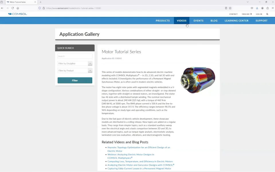
The COMSOL Multiphysics motor tutorial series demonstrates more realistic and complex electric motor models beyond the basic examples covered in earlier course sections. The series models a synchronous drive machine in 2D, 2.5D, and full 3D, with multiple model variations that progress from simple to complex configurations, including versions without rotor skewing, with rotor skewing, and with symmetry. An accompanying readme PDF describes each model version and includes plots comparing voltages, phase behavior, and torque across 2D analysis, extruded 2D analysis, and full 3D models, helping determine the accuracy and computational power required for a given application. The full transient 2D model (model 9) uses the Rotating Machinery, Magnetic interface with two magnet arrays, where the remanent flux density direction of the permanent magnets is position dependent and defined using cosine and sine functions rather than simple north and south pole assignments. The phases are modeled as single conductors—solid copper pieces—which fully resolves the skin and proximity effects rather than using a homogenized multi-phase winding. Coil voltage excitation is supplied through an added electric circuit interface, featuring phases A, B, and C connected via a star-point resistor in a star connection. Results include volumetric loss density resolved over time steps, and an evaluation group computes quantities such as average torque, electrical input power, mechanical output power, efficiency percentage, and torque ripple percentage, all with visible definitions available in the model. The 2.5D model (model 10) captures rotor skewing effects by combining different cross sections through three rotating domain features, each with an offset angle governed by a rotor position number variable that changes across domains. Periodic conditions and magnet arrays are defined with pole angles and cosine expressions that account for varying remanent flux density direction across the different sections. Simulation stability can be improved through ramping: rather than starting instantly at full rotation speed—which can cause convergence issues or artifacts—the rotation can be gradually accelerated. Beginners are advised to increase shaft speed from zero to the desired speed while adjusting phase currents accordingly, while a time ramping function offers an alternative approach. The full 3D model is significantly more complex, requiring approximately 50 hours to solve, and uses hairpin connectors while revealing end effects arising from the finite spatial dimensions of the motor—phenomena that cannot be captured in 2D simulations. The moving mesh feature handles segmented rotor sections in real space, and additional physics nodes such as gauge fixing of the zero magnetic scalar potential are involved. Volumetric loss density plots in 3D show losses in the hairpins along with end effects, demonstrating the primary advantage of 3D simulation. A dedicated course section on 3D simulation of electric motors follows. The motor tutorial series and related models are linked on the associated web page.