In accordance with our Quality Policy, COMSOL maintains a library of hundreds of documented model examples that are regularly tested against the latest version of the COMSOL Multiphysics® software, including benchmark problems from ASME and NAFEMS, as well as TEAM problems.
Our Verification and Validation (V&V) test suite provides consistently accurate solutions that are compared against analytical results and established benchmark data. The documented models below are part of the COMSOL Multiphysics® software’s built-in Application Libraries. They include reference values and sources for a wide range of benchmarks, as well as step-by-step instructions to reproduce the expected results on your own computer. You can use these models not only to document your software quality assurance (SQA) and numerical code verification (NCV) efforts, but also as part of an in-house training program.

An axisymmetric model of a rigid piston in an infinite baffle is used to exemplify the Exterior Field Calculation feature of the Acoustics Module. The radiation results provided by the COMSOL Multiphysics® software are compared to analytical results for the on-axis radiation ... Read More
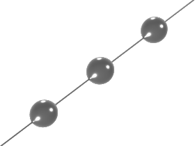
This example applies an Oldroyd-B fluid to model the thinning of a viscoelastic filament under the action of surface tension. For times smaller than the polymer relaxation time, the filament develops a beads-on-string structure. At times much larger than the relaxation time, the solution ... Read More
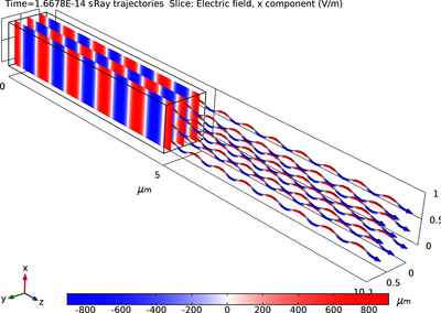
This tutorial shows how to set up a ray release based on the incident electric field at a boundary. First the Electomagnetic Waves, Frequency Domain interface is used to solve for the electric field of a plane wave. Then rays are released with initial intensity and polarization matching ... Read More
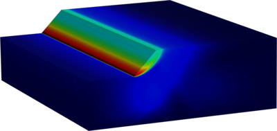
The strength reduction technique is a tool to find the factor of safety (FOS) in geotechnical problems, particularly in slope stability analyses. To determine the factor of safety of the slope, the strength properties in the Mohr–Coulomb model are gradually reduced until failure occurs. ... Read More
This example describes how to simulate the flow of a thin film of fluid in the gap between two rectangular plates, one of them with a porous facing, when the fluid is squeezed as a consequence of the relative motion between the plates. The model accounts for the ingress and egress of ... Read More

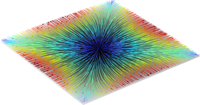
This model shows how to use the scattered field formulation to compute the transmission coefficient for impinging P and S plane elastic waves onto a finite size phononic crystal. The transmission tends to zero in the frequency range corresponding to P- and S-wave band gaps, as ... Read More

In this model, two flat end mirrors are placed at a distance and a spherical lens is inserted in the middle of the cavity. A ray is released from a point inside the cavity. Then the ray is traced for a predefined time period that is sufficiently long. Ray tracing continues until the ... Read More

This example shows a 2D steady-state thermal analysis including convection to a prescribed external (ambient) temperature. It is given as a benchmarking example. The benchmark result for the target location is a temperature of 18.25 C. The COMSOL Multiphysics model, using a default mesh ... Read More
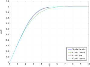
The incompressible boundary layer on a flat plate in the absence of a pressure gradient is usually referred to as the Blasius boundary layer. The steady, laminar boundary layer developing downstream of the leading edge eventually becomes unstable to Tollmien-Schlichting waves and finally ... Read More

This model shows how to implement an anisotropic, incompressible, hyperelastic material for modeling soft collagenous tissue in arterial walls. The hyperelastic material model implemented is based on the articles: Holzapfel, G. A., Gasser, T. C., & Ogden, R. W. (2000), A new ... Read More