The Application Gallery features COMSOL Multiphysics® tutorial and demo app files pertinent to the electrical, structural, acoustics, fluid, heat, and chemical disciplines. You can use these examples as a starting point for your own simulation work by downloading the tutorial model or demo app file and its accompanying instructions.
Search for tutorials and apps relevant to your area of expertise via the Quick Search feature. Note that many of the examples featured here can also be accessed via the Application Libraries that are built into the COMSOL Multiphysics® software and available from the File menu.
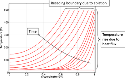
This example exemplifies how to model thermal ablation by taking into account material removal. A more detailed description of the phenomenon and the modeling process can be seen in the blog post "Modeling Thermal Ablation for Material Removal". Read More
These examples demonstrate how to use a job sequence to perform a programmatic sequence of operations, including solving; saving the model to file; and generating and exporting plot groups, results, and images. In the blog post associated with these files, "How to Use Job Sequences to ... Read More

See how to generate a mesh from scanned data via two different workflows. For both examples, the data file is imported in an Interpolation function. In the first workflow, the data is applied on a Grid dataset and a Filter dataset is used to filter out the data to represent the femur. ... Read More

Use this app to validate that the default settings correctly submit jobs to a cluster. These default settings are taken from the preferences. The app allows you to override the default cluster settings, test modifications to the current setup, and test different settings for connecting ... Read More
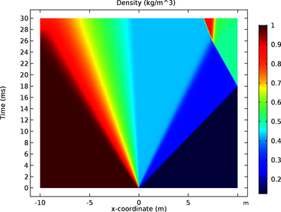
The compressible Euler equations are implemented in the Wave Form PDE interface with nodal discontinuous Lagrange shape functions to compute the flow in a shock tube. The purpose of this application is to simulate the flow in the tube and estimate the distributions of pressure, density, ... Read More

This document explains how to install and run COMSOL Multiphysics® and COMSOL Server™ with Microsoft® Azure. This requires that you have first acquired a Floating Network License (FNL) or COMSOL Server License (CSL) from COMSOL. The license manager software can run ... Read More
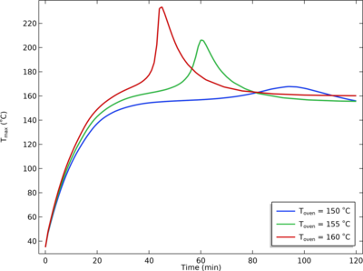
This example simulates the temperature dynamics in cylindrical battery, initially at room temperature, after being placed in an oven. As the temperature increases, various exothermal decomposition reactions are activated, which in turn result in further heating of the battery. Read More
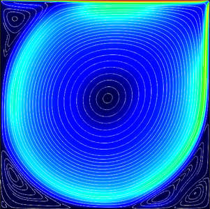
This example demonstrates how to define the lid-driven cavity benchmark in the field of computational fluid dynamics. In the model setup, a 2D square cavity has a tangentially moving wall that induces a large vortex in the center of the cavity, and small vortices in the corners. The ... Read More

These examples show how to use the tools under the Results node to generate and visualize randomized material data with prescribed statistical properties. The randomness is controlled through a spectral density distribution, which defines the spatial frequency content of the material ... Read More
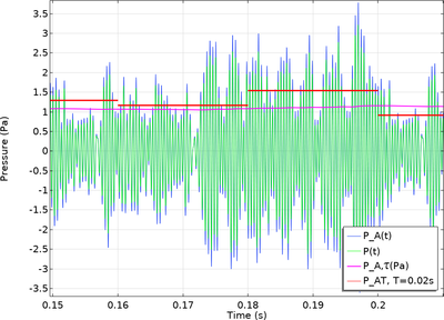
For transient acoustic problems, there are different sound pressure level metrics that have been defined in the literature and in measurement standards. These metrics are important to know when comparing results from a transient acoustic simulation to measurements from a sound level ... Read More