Modeling with PDEs: Using the Weak Form for Scalar Equations
In Part 10 of this course on modeling with partial differential equations (PDEs), we will learn about setting up PDEs in COMSOL Multiphysics® using the weak formulation. To illustrate this, we will compare using the built-in physics interfaces with that of user-defined equations defined using the Weak Form PDE interface. We will begin with how to implement the equations of electrostatics and electric currents using the Weak Form PDE interface and the test operator. We will dive into structural mechanics and plane stress in the next part of the series.
Minimizing Electrostatic Energy
The weak form of a PDE may seem a bit mysterious at first, so let us have a look at some of the theoretical background for understanding where it all comes from, starting with the electrostatics perspective.
In COMSOL Multiphysics®, when solving the equation for electrostatics, we usually apply the following form of Gauss' law:

as well as a set of suitable boundary conditions, e.g., a given surface charge density. On one part of the boundary we apply a Neumann boundary condition:

and on another part we apply a Dirichlet condition:

The Dirichlet condition represents a fixed electric potential.
An alternative way of approaching electrostatics is to consider it as a problem of minimizing the electrostatic energy over the domain  :
:

where  is the electric field and
  is the electric displacement field. Here, we will consider only a linear isotropic material. The material coefficient
  is the electric permittivity which, roughly speaking, tells us how well the material stores electric energy, and therefore how suitable the material would be to use as a dielectric in a capacitor. To get an intuition for what this minimization problem represents, you can think of a dielectric or, equivalently, an insulating domain with various metallic electrodes placed on the boundary. In many, but not all cases, the minimization problem for electrostatics can be understood as the redistribution of surface charges on the metallic electrodes so that an electrostatic energy minimum is obtained.
Minimizing this energy and adding another boundary term to the equation will eventually lead us to the weak form. First, let us recap some facts about finding stationary points in an optimization problem.
For a conventional real-valued smooth function,  , we know that we can find stationary points, which are candidate points for local maxima or minima, by setting the first-order derivative to zero:

Note, however, that there may not be any of these points if there are no conventional stationary points in the interior of the domain we are considering.
We also know that by inspecting, for example, the second- and higher-order derivatives, we can get information on whether the point is a maximum, minimum, or saddle point.
We can also understand this from the perspective of a Taylor expansion of the function around  by using a small perturbation
  :
:

This function has a stationary point when the second term in the series is zero, or:

Similarly, we can use the theory of variational calculus to expand the expression for electrostatic energy by using a small perturbation in the electric potential 

On further inspection, this expression is quite different from the Taylor expansion of the conventional function . Instead of being a real-valued function,  is a "function of a function", also known as a functional. In this case, the function
  is the electrical potential, which we assume is a field that varies throughout the domain .
To proceed from this point we also need to remember the boundary conditions:

which still need to be fulfilled for solution of the minimization problem. However, we will also require the perturbation function to be chosen so that these boundary conditions are also fulfilled for the perturbed function  . We say that is chosen to belong to a class of admissible functions with respect to the boundary conditions.
If we now expand  we get:

which is the same thing as:

where  represents the second-order terms in . In addition, because the perturbation is admissible, we can assume:

Now, similar to
the condition for stationarity comes from the first-order term in .
We can write the expansion as:

where we can define the first variation as:
 .
.
Retaining only the linear term gives:

which is called the first variation of .
However, this is not quite the full expression, or functional, that we need to minimize. To get something physically relevant, we also need to include the influence of surface charges on the boundary in the expression for the energy. When including the boundary charges we get the following, more general expression for the energy potential:

where

or

is the surface charge.
We get for the variation of the boundary term:

which leads to the following, more general condition for first-variation stationarity in the presence of surface charges:

Note that the energy potential expression is sometimes called the Dirichlet energy and the minimization method is called Dirichlet's principle.
Deriving Gauss' Law
How is this equation for the first variation related to Gauss' law, ?
To find out, we will rearrange the equation slightly and start from

For this equation to be more clear, we will set:

so that we have

Let us now perform integration by parts:

where is the computational domain and  is the boundary.
This integration by parts (or partial integration) expression should be compared with the following calculus version of integration by parts:

For more information, see https://en.wikipedia.org/wiki/Integration_by_parts.
Upon inspecting the boundary integral term

we can draw the conclusion that we can use the Neumann boundary condition:
With this, we get:

or

Since this expression needs to be valid for all admissible perturbation functions, the only possible conclusion is that

holds. With that, we have now arrived at Gauss' law by starting from the minimization of electrostatic energy.
Note from the derivation above that the Neumann boundary condition enters naturally in the equation.
So, what about those parts of the boundaries where we have the Dirichlet condition ?
We can handle this type of boundary condition, on those boundaries where it applies, by adding a virtual surface charge (a virtual flux):

where we adjust this virtual surface charge, which, in general, is spatially varying on the boundary, so we get .
In a practical implementation, such a virtual surface charge can be applied by means of, for example, Lagrange multipliers. For more information on Lagrange multipliers, see the COMSOL documentation and our blog post on methods for dealing with numerical issues in constraint enforcement.
The Weak Form of a PDE
For handling general PDEs, the approach of minimizing energy using variational calculus does not work since a PDE may not correspond to an energy minimum but instead to a saddle point. To proceed, we focus on the last step in the derivation:

and generalize the idea that this expression needs to be valid for all admissible perturbation functions  .
.
Let us now see how we can start with a PDE, such as Gauss' law, and derive its weak form. This procedure can be generalized to a great variety of PDEs and system of PDEs.
Starting with the Gauss' law PDE:
with a Neumann boundary condition:
we multiply the PDE with an admissible function — from now on called a test function — and integrate over the domain:

We will see later how we can introduce test functions in the equation-based user interfaces by using the dedicated test operator.
Next, perform integration by parts and use the boundary condition to get the weak form of Gauss' law:

Note that this is just the earlier derivation backward.
Now, what are some of the benefits of using the weak form as opposed to the original strong form of the PDE?
One benefit is related to the derivative orders. When implementing this using the finite element method, the solution is approximated with piecewise polynomial functions. By using integration by parts, we have decreased the order of the derivatives in the equation. The original equation had second-order derivatives in space, whereas the weak form only has first-order derivatives. This fact enables us to use lower-order polynomials that would otherwise be impossible to use if implementing a solution method based directly on the strong form of the PDE. This can make the implementation easier and more efficient.
Another benefit comes from the fact that the weak form of the PDE is defined in the integral sense instead of pointwise. The equation
can be made valid in a mathematically consistent way even if there are discontinuities present, such as jumps in the material coefficient or in the boundary conditions. Even if such discontinuities are present in the solution itself, the weak form of the equation is still valid.
A solution to the weak form is also called a weak solution, as opposed to a strong solution to the original PDE. Alternatively, we can say that the solution exists in the weak sense. Allowing for discontinuities is very important in order to model real-world scenarios. The notions of weak equation form and weak solution can be made mathematically precise; use the links attached here to learn more.
Behind the scenes, COMSOL Multiphysics® will automatically convert any equation implemented using the Coefficient Form PDE or General Form PDE interfaces into a weak form of the PDE. The Weak Form PDE interface enables you to enter the equations directly on the weak form, which can be convenient. Many of the built-in physics interfaces are also based on the weak form, and you can even inspect and modify these; see Part 11 for more information.
Electric Currents as a Weak Form PDE
The PDE for electric current conservation is similar to that of electrostatics:

Here, the material coefficient is the electric conductivity,  . We also have a right-hand-side source term
  , which represents some injected current density from an external source, such as an electrochemical reaction.
The corresponding energy functional that needs to be minimized is:

In the equation, is the electric field,  is the current density in the domain, and
  is the current density flowing through the boundary. This expression is essentially the same type of energy expression as in the electrostatics case.
Note that since the electric currents equation represents a stationary PDE, the total power loss can be converted into total energy loss by simply multiplying with an arbitrary time interval. In SI units, this corresponds to converting from watts to joules.
The electric currents PDE has an associated set of boundary conditions for a given current density, , as a Neumann boundary condition:

on some part of a boundary. There is also a fixed electric potential,  , as a Dirichlet condition:
on other parts of the boundary.
The corresponding weak form of this PDE is:

Note that the source term does not change during the partial integration step.
By convention, the Weak Form PDE interface assumes that the equations are all moved to the right-hand side, so the equation we want is:

In a similar way, you can implement any version of Poisson's equation or diffusion-like conservation laws using the Weak Form PDE. As a matter of fact, you can implement any equation that you can formulate using the Coefficient Form PDE or using the Weak Form PDE. This is also true for the General Form PDE.
Point Charges and Point Sources
Being able to formulate and solve equations on the weak form makes it possible to work with point charges or, more generally, point sources. For example, we might have a point charge to Gauss' law:

where  is the Dirac delta function assigning a unit charge to the origin. Note that the delta function is not related to the use of the same symbol used in the variational calculus derivations earlier. This PDE does not have any solution in the usual strong sense, but it is perfectly sound in the weak sense. More generally, we can write:

where is the charge at the origin.
When we formulate this as a weak equation we get:

The last term assigns a unit charge to the origin. We can also write this as:

where  is the value of the test function at the origin.
For an example of this, see the Implementing a Point Source model.
Implementing Electric Currents Using the Weak Form
We will now look at how to implement the equations for the built-in Electric Currents interface using the Weak Form PDE interface.
For this example, we will reproduce the pacemaker electrode tutorial model from the application libraries (shown below). In this example, you can also find documentation for building this model completely from scratch, including step-by-step instructions.
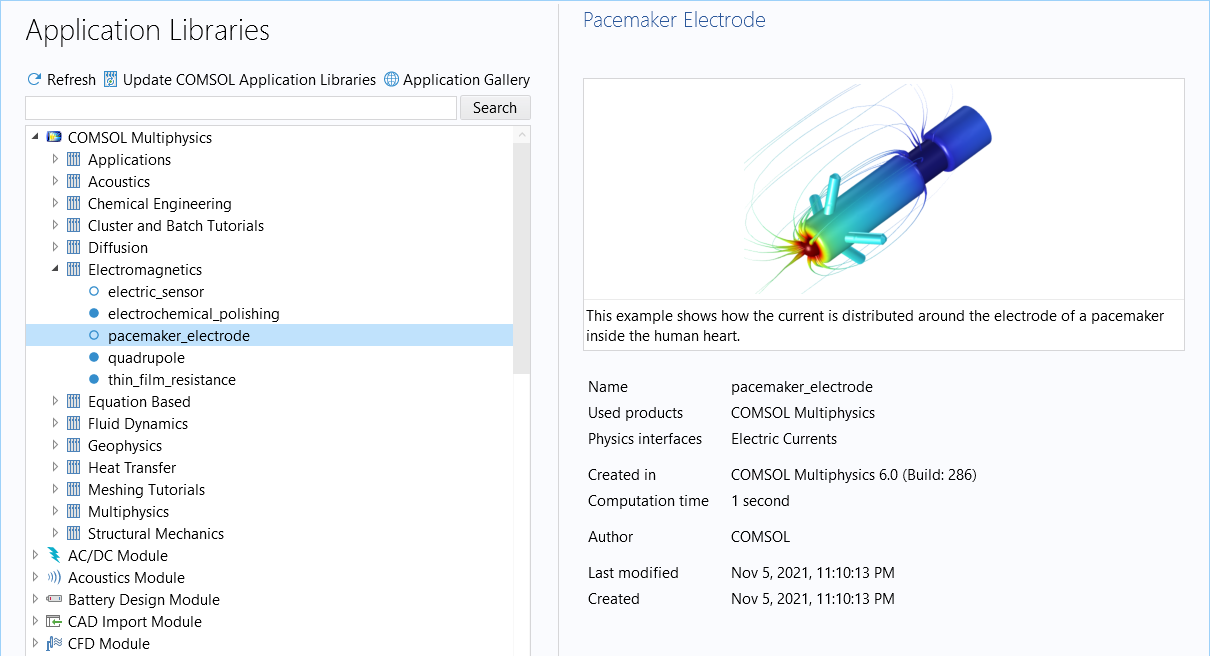
The Application Library with the pacemaker electrode tutorial model selected.
In the Model Wizard, select the Weak Form PDE interface, and change the Field name and Dependent variable name to V, and then change the units. For the units, select Electric potential (V) and enter a custom A/m3 unit for the Dependent variable quantity, V, and source term quantity, respectively.
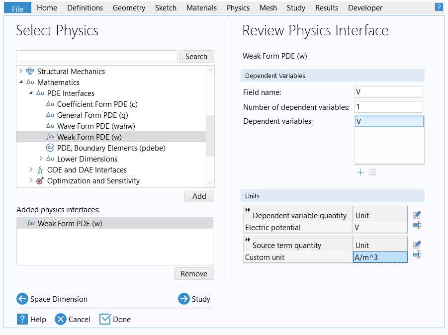
The physics settings in the Model Wizard for implementing electric currents using the Weak Form PDE interface.
For this example, select a Stationary study and then import the geometry after downloading it here.
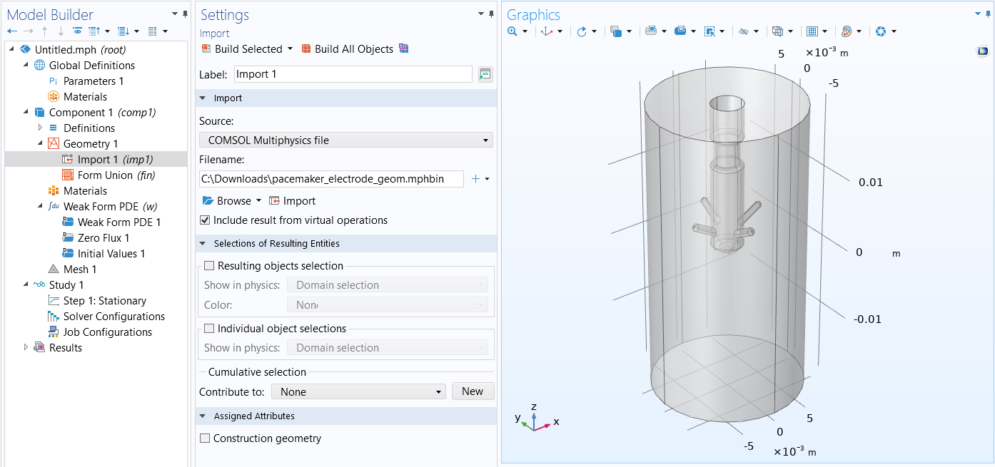 The Model Builder with Import feature selected, the corresponding Settings window, and the Graphics window showing the pacemaker electrode geometry.
The imported pacemaker electrode geometry.
The Model Builder with Import feature selected, the corresponding Settings window, and the Graphics window showing the pacemaker electrode geometry.
The imported pacemaker electrode geometry.
The weak form equation that we want to implement is:

In this example, we will not have a source term, so we have that  .
.
How do we enter the weak form in the user interface? We do this by using the test operator. For example, if our dependent variable is V, then the syntax for the corresponding test function is test(V). In the user interface, you enter the integrands for the boundary and domain in separate text fields.
Starting with the domain integrand:

Using the test operator, you can enter the domain integrand in the user interface as:
(-(test(Vx)*Vx+test(Vy)*Vy+test(Vz)*Vz))*sigma
where test(Vx), test(Vy), and test(Vy) are the gradient components of the test function  . In Part 11 of this series, we will learn more about the test operator.
The figure below shows how the weak expression appears in the Weak Form PDE interface.
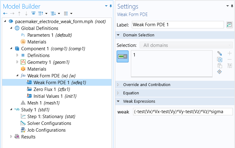
The weak form expression for the Pacemaker Electrode example.
The material property sigma is defined as a global parameter, as shown in the figure below.
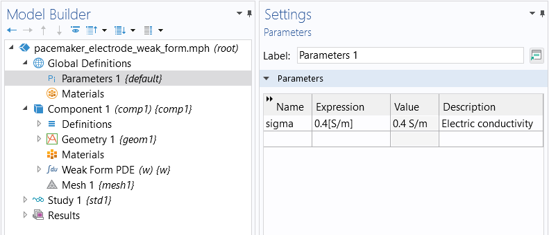
The material property for the electric conductivity.
For the boundary conditions, we have a Dirichlet Boundary Condition  on 4 surfaces, as shown in the figure below. This corresponds to a Ground boundary condition in the built-in physics interface for electric currents, the Electric Currents interface.
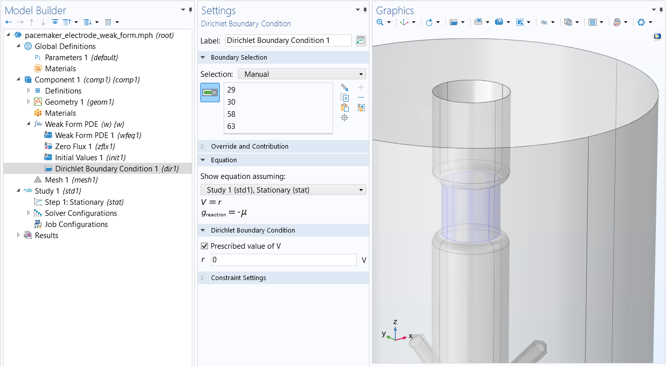 The Model Builder with the Dirichlet Boundary Condition selected, the corresponding settings, and the Graphics window showing a close-up of the model.
The boundaries that are grounded.
The Model Builder with the Dirichlet Boundary Condition selected, the corresponding settings, and the Graphics window showing a close-up of the model.
The boundaries that are grounded.
At the tip of the electrode, we will add another Dirichlet Boundary Condition  on 4 surfaces, as shown in the figure below. This corresponds to an Electric Potential boundary condition in the predefined physics interface for electric currents.
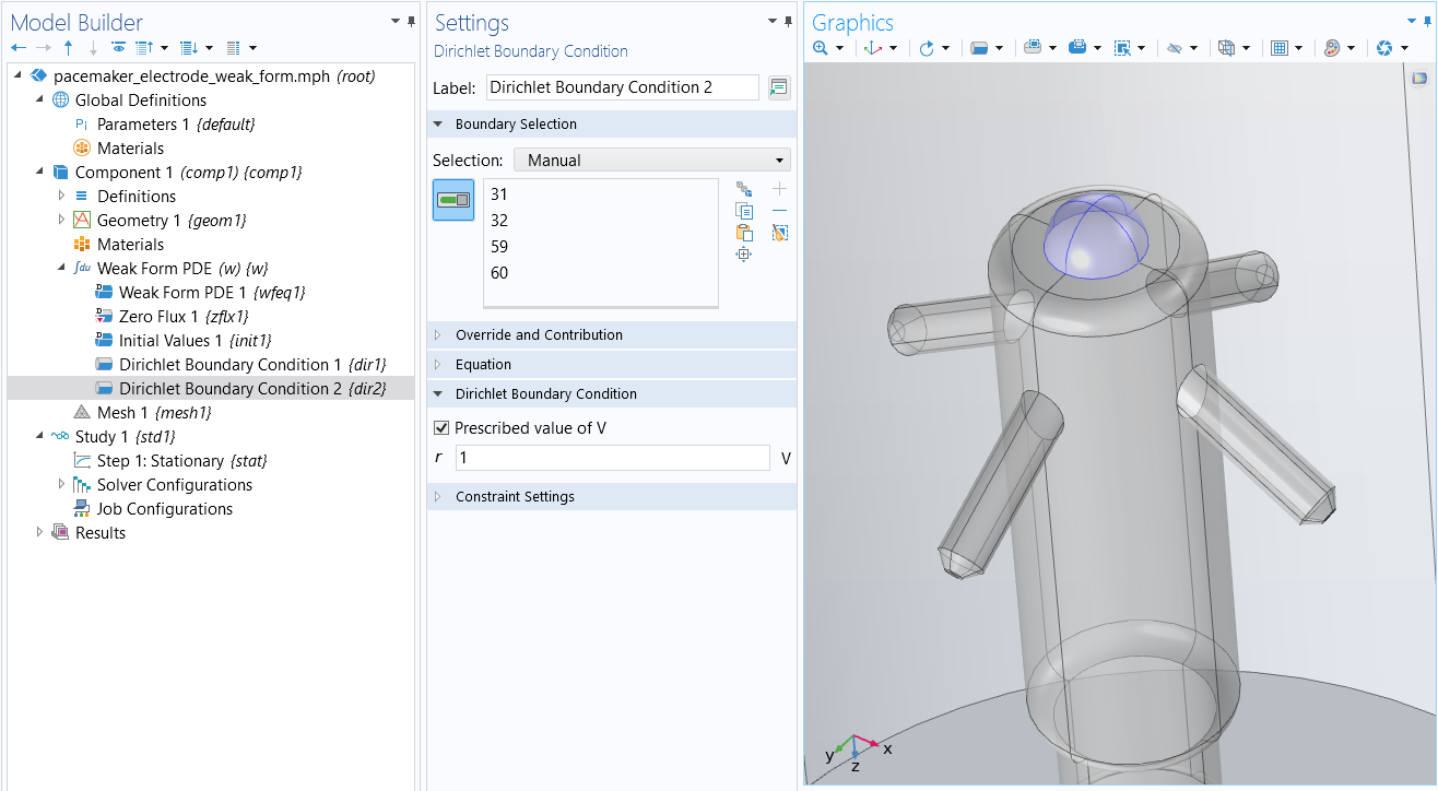 The Model Builder with a second Dirichlet Boundary Condition selected, the corresponding Settings window showing the prescribed value of V, and the Graphics window showing the tip of the model.
The boundaries with an applied electric potential.
The Model Builder with a second Dirichlet Boundary Condition selected, the corresponding Settings window showing the prescribed value of V, and the Graphics window showing the tip of the model.
The boundaries with an applied electric potential.
There will be no other types of boundary conditions used in this example. However, if you wanted to also set the surface charge density, you would do so using the Flux/Source boundary condition.
After computing, you get a default plot of the dependent variable, V, as shown in the figure below.
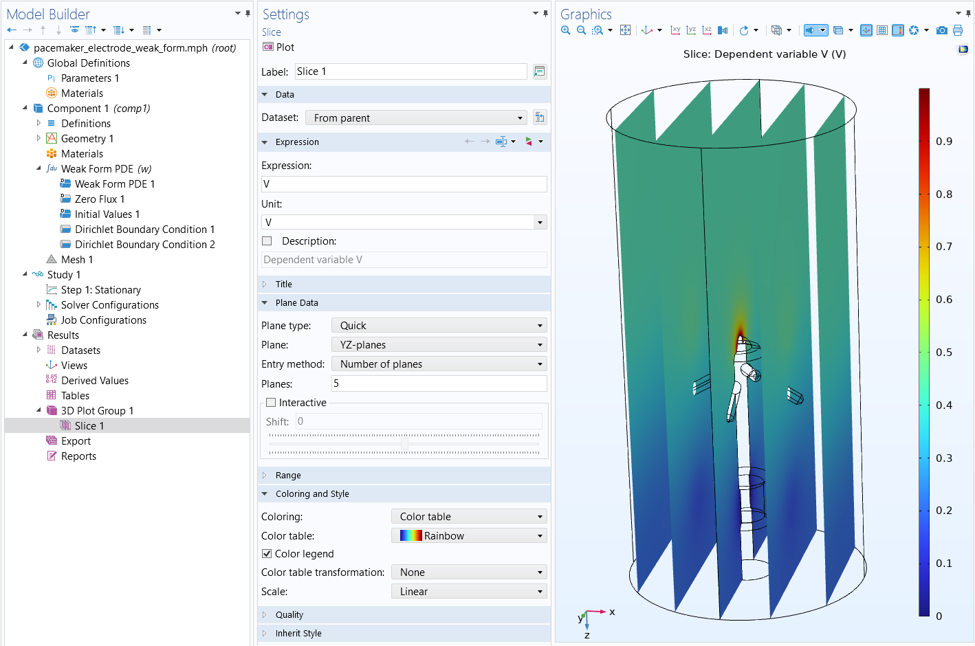 The Model Builder with a slice plot selected, the corresponding Settings window, and the Graphics window showing the model in the Rainbow color table, where the model is mostly blue and green.
The electric potential visualized as a slice plot.
The Model Builder with a slice plot selected, the corresponding Settings window, and the Graphics window showing the model in the Rainbow color table, where the model is mostly blue and green.
The electric potential visualized as a slice plot.
Just like with the previous examples in this course, you can now define variables for quantities, such as the electric field components, the current density components, and so on.
Further Learning
The model example used in this article is available for download, though we encourage you to build the model from scratch following the guidance in this article. You can open and compare the model files for both the version of the model built using the Weak Form PDE interface as well as the version built using the software's predefined physics interface, available in the Application Library. This will reinforce how to set up PDEs in COMSOL Multiphysics® using the weak form of equations.
Additionally, there are multiple blog posts that discuss the concept of the weak formulation, implementing it in the software, how the weak form equations are discretized, and more:
- A Brief Introduction to the Weak Form
- Implementing the Weak Form in COMSOL Multiphysics
- Discretizing the Weak Form Equations
- Implementing the Weak Form with a COMSOL App
Submit feedback about this page or contact support here.