

In the first part of this blog series, we discussed how to solve variational problems with simple boundary conditions. Next, we proceeded to more sophisticated constraints and used Lagrange multipliers to set up equivalent unconstrained problems. Today, we focus on the numerical aspects of constraint enforcement. The method of Lagrange multipliers is theoretically exact, yet its use in numerical solutions poses some challenges. We will go over these challenges and show two mitigation strategies: the penalty and augmented Lagrangian methods.
Using a Lagrange Multiplier for a Global Constraint
Consider finding the shape u(x) of a uniform catenary of a specified length. A catenary of uniform density per unit length hanging under its own weight minimizes the functional
If the only constraints we have are boundary conditions, this problem is free to adjust the length of the catenary to get the lowest potential energy satisfying the end conditions. However, if we require the catenary to have a specified length l, this introduces the global constraint
As discussed in Part 2 of this series, this constrained minimization problem can be turned into an unconstrained minimization problem with a new degree of freedom for the Lagrange multiplier.
Remember that a global constraint has a single Lagrange multiplier per constraint instead of a field, as in distributed (pointwise) constraints. Let’s generalize at this point and use F = u(x)\sqrt{1+u^{\prime}(x)^2}, \qquad g = \sqrt{1+u^{\prime}(x)^2}.
We derive the first-order optimality conditions by setting the first variational derivatives of \mathcal{L}[u(x),\lambda] to zero, with respect to both u(x) and \lambda. Refer to Part 1 of the series for more information on variational derivatives.
Let’s now solve for the shape of a catenary hanging on two poles that are 10 meters and 9 meters high, respectively, and located 10 meters apart. Additionally, we want the catenary to be 10.5 meters long.
The two Dirichlet boundary conditions at the ends can also be added here as constraints with their own Lagrange multipliers. We showed how to do this in Part 2. Here, let’s focus on the global constraint. We will use the built-in Dirichlet Boundary Condition node to fix the ends.


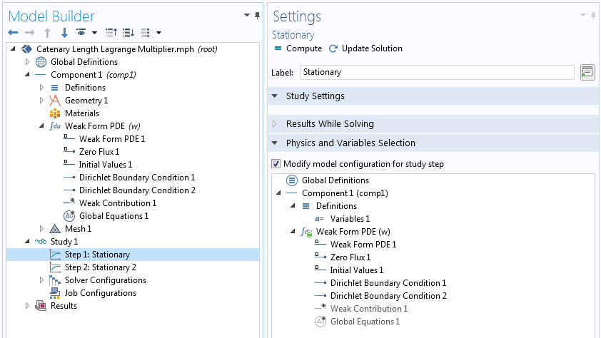
Implementing a global constraint.
Note in the above weak contribution that we have not included the term containing \frac{\partial g}{\partial u}, because g is only a function of u^{\prime} and not u.
Attempting to compute the solution generates an error message. This arises from a common numerical problem when solving nonlinear problems containing global or distributed constraints using the method of Lagrange multipliers. The finite element stiffness matrix (the Hessian of the optimization problem) can be singular for some trial solutions. As such, it becomes necessary to start from a good initial guess.
One common way to overcome this challenge is to use the solution of the unconstrained problem as an initial estimate for the constrained solution. In the COMSOL Multiphysics® software, this can be achieved by adding two steps within the same study and disabling the constraints in the first study. The solution of the first step will automatically be used as an initial iterate in the second step.
Using an unconstrained solution as an initial estimate for a constrained problem.
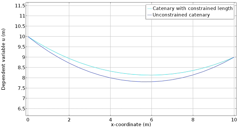
A catenary with constrained length.
If we evaluate intop1(g) in Results > Derived Values > Global Evaluation, we see that the length is exactly 10.5 meters. The Lagrange multiplier is also available in Global Evaluation. Physically, this Lagrange multiplier is related to the tension we have to apply to keep it taut at the desired length.
Another common numerical problem with Lagrange multipliers is the loss of positive definiteness in the stiffness matrix. Many unconstrained variational problems have positive definite stiffness matrices. As such, iterative linear solvers, which exploit positive definiteness, can be used. Using Lagrange multipliers for constraint enforcement leads to saddle point problems, and the corresponding linear systems are indefinite. This is not an insurmountable hurdle, as direct solvers can be used — It may just be computationally expensive.
Several methods have been devised to avoid the numerical downsides of Lagrange multipliers in global and distributed constraints. Here, we discuss two of the most widely used options: the penalty method and the augmented Lagrangian method.
The Penalty Method
A penalty reformulation of a constrained minimization problem replaces the Lagrange multiplier term by a term that penalizes constraint violation. In the case of the global constraint, we have the penalized objective function
If the penalty factor \mu is large, the second term in the above equation makes the penalty term so large that satisfying the constraint becomes necessary to minimize the total functional. We take the square of the constraint violation so that both undershooting and overshooting of the length are penalized. As such, this is a two-sided constraint. In contrast, inequality constraints are one-sided.
Here, the penalty factor is something we pick, thus the only unknown is u(x). The first-order optimality condition thus becomes
Compared to the Lagrange multiplier method, we can see that this approach is akin to approximating the Lagrange multiplier by a proportionality constant multiplied by the constraint violation.
If we think of the Lagrange multiplier as the force needed to keep the constraint, the penalty method provides a linear spring that pushes back when the constraint is violated, and we decide the spring constant. If our constraint is temperature, for example, the penalty method provides a heat flux proportional to the difference between the trial temperature and specified temperature, and we decide the heat transfer coefficient.
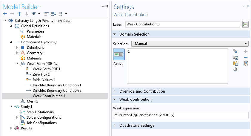
Example of the penalty enforcement of a global constraint.
The penalty method is easy to implement and has attractive numerical properties. It does not add new degrees of freedom and keeps the positive definiteness of the stiffness matrix if the unconstrained stiffness matrix was positive definite. However, it has its own cons. For instance, the constraint is not satisfied exactly. To do so, we need to make the penalty parameter infinity, but we can’t do that numerically. In fact, a finite but very big penalty term can make the numerical problem ill-conditioned. Additionally, a very large penalty parameter makes the solution focus too much on feasibility at the cost of optimality. Thus, the trick is to find a penalty parameter big enough to better approximate the constraint — but not too big.
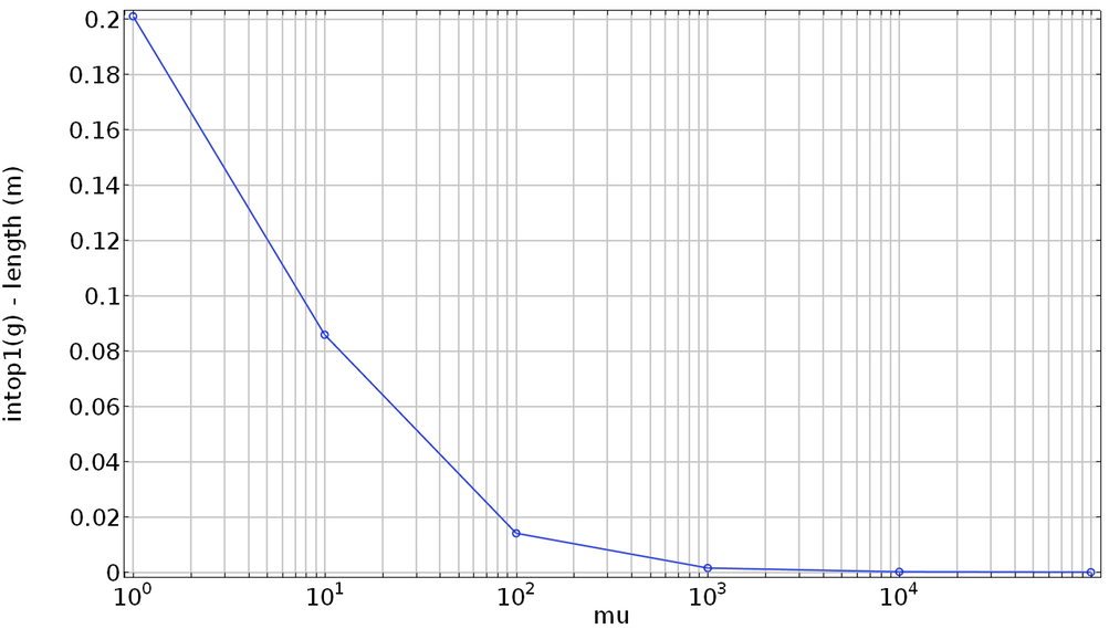
Let’s see how good the length constraint is satisfied for various values of the penalty parameter.
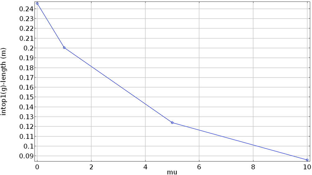
With a higher penalty parameter, the difference between the computed and specified lengths gets closer to zero.
As we can see from the above plot, a higher penalty factor enforces the constraint better. However, if we try a penalty factor of 20, we get a convergence error because the penalty factor is too high.
An Auxiliary Sweep of Penalty Parameters
Some algorithms have been developed to sequentially improve the penalized problem. One such simple algorithm is to gradually increase the penalty factor while reusing the converged solution from a previous penalty parameter as an initial estimate.
The approximate Lagrange multiplier contains a product of the constraint violation and the penalty term. As such, when the constraint violation is small, we can afford to use a large penalty parameter without making the numerical problem ill-conditioned. Thus, if we start from a trial solution whose solution approximately satisfies the constraint, we can use higher penalty factors (compared to a trial solution that violates the constraint by a large amount). This strategy can easily be implemented in COMSOL Multiphysics by adding an Auxiliary Sweep over the penalty parameter.
Difference between computed and specified lengths versus penalty factor when an auxiliary sweep over penalty factors is used.
As demonstrated by the above graph, using an auxiliary sweep over the penalty factor enables us to use a much higher penalty factor without ill-conditioning and, more importantly, enforce the constraint better. The plot below compares the solution from these continuation solutions and the Lagrange multiplier solution, which is exact.
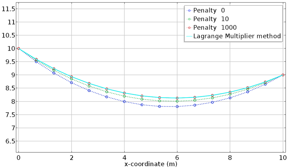
Comparison of the penalty and Lagrange multiplier solutions.
The Augmented Lagrangian Method
The augmented Lagrangian method was devised to combine the pros of the penalty and the Lagrange multiplier methods while avoiding the cons. For clarity, let’s start with a problem from calculus.
Consider the problem
The Lagrange multiplier method works with the unconstrained problem
whereas the penalty method uses
The augmented Lagrangian method has both the Lagrange multiplier and penalty terms.
Whereas in the Lagrange multiplier method, we take the Lagrange multiplier as an unknown, in the augmented Lagrangian method, we start with an estimate of the Lagrange multiplier and iteratively improve it.
The first-order optimality condition for the augmented Lagrangian function is
Comparing this with the optimality condition for the Lagrange multiplier method shows that an improved estimate for the multiplier is
Going back to the variational calculus and the global constraint we are discussing today, the augmented Lagrangian iteration is
\left(\lambda_k + \mu \left[\int_a^b g(x,u,u’)dx – l \right]\right)
\int_a^b \left[\frac{\partial g}{\partial u}\hat{u}+\frac{\partial g}{\partial u’}\hat{u’}\right]dx, \qquad \forall \hat{u}.
This iteration continues until the constraint violation is small enough (or equivalently, until the multiplier stops changing appreciably). The initial Lagrange multiplier is often taken to be zero. Keep in mind that the solution u is indexed by k as well. It is left out of the equation above to focus the attention on the Lagrange multiplier updates.
By gradually accumulating more and more of the forces (fluxes) in the Lagrange multiplier, this method enforces the constraints well while keeping the penalty parameter small. The augmented Lagrangian method is particularly attractive for distributed constraints, as each point can update differently based on local conditions.
The penalty method (without the sequential increase) and the augmented Lagrangian method are built-in methods for contact constraints in COMSOL Multiphysics, but contact mechanics involves inequality constraints. In the next blog post in this series, we will show how to add user-defined inequality constraints in the event that there is no built-in feature for the corresponding physics.
Deliberate Constraint Violation
Sometimes we want to deliberately violate constraints. Say we want to set the length constraint to 10.04 meters in the above example. This is physically impossible, since the shortest distance (straight line distance) between the supports is 10.05 meters.
The Lagrange multiplier method wants to enforce the constraint exactly, and as such, this will lead to a convergence problem. However, we may still want to live with some violation of the constraint to obtain an inexact solution. In such cases, with inconsistent constraints or when there are redundant constraints, the Lagrange multiplier method rightly cannot converge. However, we can use the approximate constraint enforcement methods, such as the penalty and augmented Lagrangian methods, to relax the constraints and obtain a “nearby” solution. For example, the Multibody Dynamics Module provides a built-in penalty method for joints to make the models less sensitive to over-constraints.
Coming Up Next…
Today, we have shown that the Lagrange multiplier method works exactly…when it works. However, it is more sensitive to initial estimates of the solution and can turn a potentially definite problem indefinite, necessitating the use of direct solvers. The penalty and augmented Lagrangian methods overcome these challenges in exchange for some violation of the constraints.
We wish we could enforce constraints exactly, but in problems with inconsistent or too many constraints, we may want to enforce constraints inexactly to obtain some approximate solution. In the next blog post, we will discuss inequality constraints. The Lagrange multiplier method comes with an extra downside for inequality constraints.
We will spend more time in this series on the penalty method, but that will conclude our discussion of one dimensional and single unknown problems. In another upcoming blog post, we will generalize to multiple dimensions, multiple fields, and higher-order derivatives.
Contact COMSOL to learn more about the equation-based modeling features of COMSOL Multiphysics by clicking the button below.


Comments (4)
Petr Henyš
September 11, 2018Hi!
nice tutorial, but what about Nitsche’s method for enforcing constraints? Can we implemented it in Comsol?
Thanks,
Petr
Temesgen Kindo
September 12, 2018Thanks for your comment Petr.
COMSOL Multiphysics already has weak enforcement of constraints built-in. When you specify boundary conditions, for example, you have the option of “use weak constraints” in the Constraint Settings section of the boundary condition’s settings window. Please check the COMSOL Reference Manual for what the various options there do.
If your goal is to just weakly enforce constraints, it is already there in COMSOL Multiphysics. But if there is a specific numerical strategy you want to follow, we suggest you contact our support team with details. The answer here is a qualified yes. As the literature has several variants of Nitsche’s method, however, we would have to know the specific formulation you have in mind before giving a definite answer. The technical support team can be reached via support@comsol.com.
Cheers,
Temesgen
Ivan Melikhov
September 13, 2018Hello Temesgen!
Thank you for this great blog series! Could you suggest where I can found details (or example) of COMSOL implementation of the augmented Lagrangian method?
Thank you,
Ivan
Temesgen Kindo
September 13, 2018Hi Ivan,
Thank you for the comment.
There are two things you want to take care of in the augmented Lagrangian method. First you want to have a history variable which stores the Lagrange multiplier from the previous converged step (say step k). This can be done by adding a global or domain algebraic equation. Second you want to make sure that during the iteration for the nonlinear solution (step k+1) you use the Lagrange multiplier from the previous converged step and not from the previous algebraic iteration. This can be done with a previous solution operator or more cleanly by adding the Lagrange multiplier variable to a Lumped Step in the Solver Configuration.
We do not have an example in our Application Gallery that shows this. The built-in augmented Lagrangian features such as in contact mechanics do this internally and you won’t see much of it. But we can make you an illustration model, say to solve the example in this blog, if you contact the Technical Support team.
Cheers,
Temesgen