Learning Center

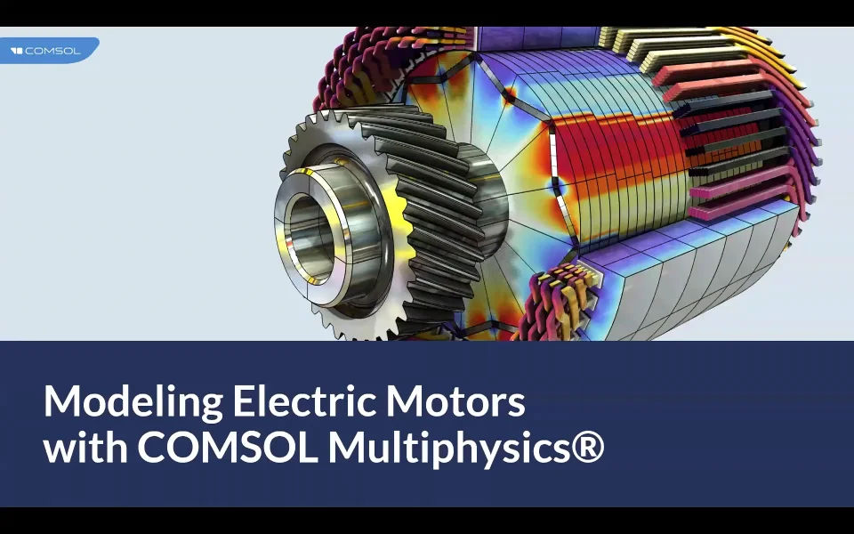
This course, Modeling Electric Motors with COMSOL Multiphysics, is a six-part series that begins with a general introduction to electric motor modeling and progresses to more advanced topics. Subsequent parts cover double-checking and debugging motor models, sector modeling, demonstrations from the motor tutorial series featuring industrial-scale models, time periodic motor modeling, and 3D motor modeling. Electric machine modeling in COMSOL supports 2D, 3D, and 2.5D geometries, with numerous tutorial models, material models, and options for windings and circuits. A key benefit of COMSOL is its multiphysics capability. Electromagnetics form the foundation of electric motor modeling and can be coupled with heat transfer to observe motor heating, structural mechanics to evaluate stress and forces, acoustics to assess sound levels, and CFD simulations. Optimization algorithms are also included, enabling a holistic motor design process within a single modeling environment. COMSOL supports various device types, including radial flux, axial flux, linear, and transverse flux machines. The fundamental 2D modeling workflow uses the Rotating Machinery, Magnetic interface within the AC/DC branch, beginning with a stationary study. The workflow involves defining parameters, drawing or importing geometry, assigning materials, applying physics, meshing, solving, and reviewing results. Geometries can be imported as CAD files, drawn directly in COMSOL, or built from predefined part libraries such as surface mounted magnet rotors and slotted stators. Critically, the geometry must be finalized with a Form Assembly rather than a Form Union, which creates an identity boundary pair between rotor and stator, enabling a sliding mesh that prevents mesh distortion during rotation. Only one identity boundary pair should exist at the rotor-stator interface. Materials are assigned using selections, and nonlinear soft iron materials use BH curves, while permanent magnets are defined with recoil permeability and remanent flux density. Rotation is applied through the Moving Mesh feature using a Rotating Domain with constant angular velocity. Within the Rotating Machinery, Magnetic interface, conducting magnets are assigned with north and south poles arranged in an alternating circular pattern, laminated cores use a Steinmetz loss model with out-of-plane lamination and a stacking factor, and multi-phase windings are configured with automatic three-phase layouts, phase currents, and homogenized conductor treatment. The Arkkio torque method, a numerically stable volume integral over the air gap, calculates torque. Best practice recommends at least two mesh elements across the air gap for good continuity between rotor and stator, and measuring the air gap distance helps set consistent mesh sizing. A stationary study with an initial angle sweep identifies the angle producing maximum torque, followed by a time-dependent study using the stationary result as initial values to ensure numerical stability with permanent magnets. Probes allow monitoring of electromagnetic torque during solving, and results include animations, cycle-averaged losses via a time-to-frequency losses study, and Fourier analysis of torque ripple harmonics. A common mistake to avoid is neglecting correct parameter units when sweeping angles or rotational frequencies. The next part of the course addresses debugging and double-checking motor models.