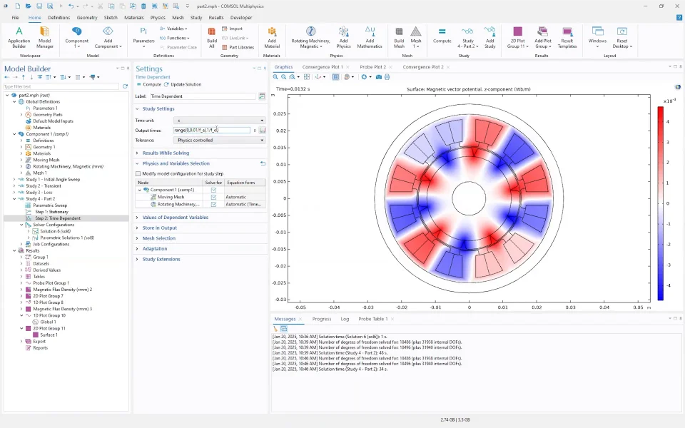
Simulation results from a motor model may not align with expectations. When this happens, it becomes necessary to debug your model and ensure the results are valid. In this video, we will demonstrate several debugging strategies that may be used if, for example, the torque ripple, or the losses, or the magnetic fields do not look as expected. Debugging motor models has some similarities with debugging other finite element models, so you may be able to apply prior experience if you have it. You may want to pay particular attention to some of the following areas: your materials, magnet and winding configurations, physics couplings, mesh refinement, and solver settings.
Watch the video below to walk through some common steps you can take to debug your motor models.
Tutorial: Motor Model Debugging and Double Checking
Press O for more options
25:58
Introduction to Debugging Motor Models
General Debugging Strategies
Motion and Stationary Study Checks
Verifying Magnet Configurations
Checking Multiphase Winding Currents
Torque and Mesh Refinement Studies
Analyzing Induced Voltages
Analyzing Magnetic Vector Component Az
Final Steps in Solver Configuration
Exploring Solver Settings
Understanding Coupled Node Methods
Final Insights on Solver Configurations
This second part of the course Modeling Electric Motors with COMSOL Multiphysics focuses on debugging and double-checking a motor model when torque ripple, losses, or magnetic fields do not appear as expected. Debugging a motor model follows the same general principles as debugging any finite element simulation. The first check involves the materials: nonlinear BH curves create nonlinearities that are harder for solvers to handle than linear materials. Temporarily assigning linear materials such as iron helps determine whether convergence problems are material related. For user-defined BH curves, the BH Curve Checker, available in the Application Library under the AC/DC Module, loads a curve, optimizes jagged or stepped curves into smoother ones, and improves solver convergence.
Isolating the source of a problem is a key strategy. Running a stationary study and sweeping a rotation angle reveals whether issues arise from the transient motion or already exist in the static case. Similarly, comparing a single-physics Rotating Machinery, Magnetic interface against setups using an electric circuit interface or other multiphysics couplings shows whether the problem originates from excitation or coupling. Conducting magnet features should be verified by computing initial values and plotting the remanent flux density with an arrow surface plot; a correct circular arrangement shows magnets alternating upward and downward as intended, which is especially important to confirm for custom magnetization patterns such as Halbach arrays.
The multiphase winding and current excitation are checked using probes and surface plots of the current in the z direction, applying a selection to the stator slots and using the Wave Light Classic color scale with red for positive, blue for negative, and white for zero. Disabling result smoothing (no refinement) shows the actual computed currents. Plotting the winding phase currents globally should show a clean sinusoidal signal with the prescribed peak current and a 120-degree phase offset. A mesh refinement check involves introducing a factor variable multiplied by both the peak current and the electrical conductivity, then setting it to zero in a parametric sweep so the torque should ripple around zero; a small offset indicates the mesh or solver tolerance can be refined. Induced voltages, which appear when currents are set to zero, provide another verification of the winding pattern and should show sinusoidal amplitudes with balanced positive and negative values and a 120-degree phase shift. Plotting the out-of-plane vector potential Az on the spatial frame, so edges move with the rotor, confirms that red and blue regions remain aligned and balanced throughout rotation.
Only after materials, rotation, magnets, excitation, and mesh have all been verified should solver configurations be adjusted, since most motor model issues stem from incorrectly set up physics rather than the solver. Useful solver adjustments include increasing the number of output times for finer resolution, keeping time stepping set to strict so the solver takes at least the provided steps, setting a small initial step to initialize the solver, retaining the automatic Newton method with automatic damping in the fully coupled node, increasing the maximum number of iterations beyond the default of ten, and making termination more rigorous by requiring both solution and residual criteria. In general the default solver settings are sufficient.
This website stores cookies on your computer. These cookies are used to collect information about how you interact with our website and allow us to remember you. We use this information in order to improve and customize your browsing experience and for analytics and metrics about our visitors both on this website and other media. To find out more about the cookies we use, see our Privacy Policy.
If you decline, your information won’t be tracked when you visit this website. A single cookie will be used in your browser to remember your preference not to be tracked.