

The Oldroyd-B numerical model defines flow in fluids that exhibit complex viscoelastic behavior under strain, such as clay, toothpaste, oil, and polymer solutions. In a benchmark model of an Oldroyd-B fluid, the COMSOL Multiphysics® software and add-on CFD Module are used to solve the numerical model, the results of which have been validated by published research.
The Oldroyd-B Model Defines Viscoelastic Fluid Behavior
The Oldroyd-B model can be written as an equation that describes viscoelastic fluid behavior with the following variables:
- Stress tensor
- Relaxation time
- Retardation time
- Upper-convected time derivative of the stress tensor
- Fluid velocity
- Total viscosity composed of solvent and polymer components
- Deformation rate tensor or rate of strain tensor
Although the model seems simple, there are many cases in which it can be a challenge for numerical simulation due to the complex fluid dynamics involved. This is where the COMSOL® software comes in…
The Weissenberg Number and Least-Squares Stabilization
The dimensionless Weissenberg number compares the elastic and viscous forces in an Oldroyd-B fluid. In simple cases, such as a steady-state shear flow, this number is found by multiplying the shear rate by the relaxation time.
What does the Weissenberg number tell us about a fluid’s behavior?
- 0 means the fluid is purely viscous
- Greater than 1 is considered high for an Oldroyd-B fluid
- An infinite number means the fluid gives a purely elastic response
We know that the Weissenberg number is important for analyzing Oldroyd-B fluids, so what’s stopping us from finding it? The Weissenberg number is convective by nature. This means that as the fluid increases in elasticity, the solution becomes more unstable.
The material model in this tutorial is defined using equation-based modeling, since there is no Oldroyd-B interface yet in the CFD Module. Therefore, the least-squares stabilization terms that stabilize the numerical solution have to be added manually. Doing so improves the solution stability and enables us to find solutions over a larger range of Weissenberg numbers before they become unstable.
Numerical Modeling of a Viscoelastic Fluid
The geometry for the Oldroyd-B benchmark consists of a cylinder between two parallel plates with a 2D flow of an Oldroyd-B fluid. One specification to note is that there is a 1:2 aspect ratio between the cylinder’s radius and the half-width of the channel. Also, the computational domain is set to be 40 times longer than the half-width, which enables you to avoid entrance and exit effects.
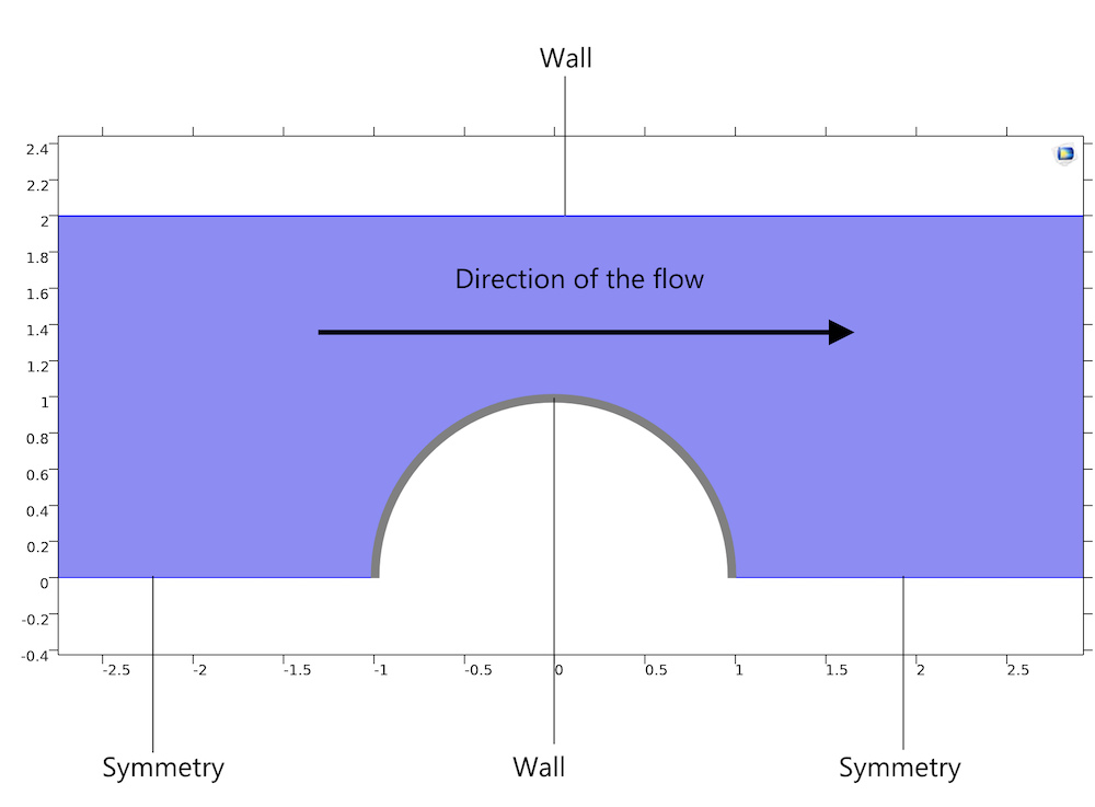
A schematic of the Oldroyd-B fluid flow model for describing viscoelastic behavior.
The model includes the following boundary conditions:
- Symmetry, so you only need to model the upper halves of the channel and cylinder
- No-slip boundaries on the walls
- Half-inlet, with the developed parabolic velocity profile and corresponding extra stress components specified
- Pressure at the outlet to account for the developed flow
By solving the model parametrically, you can gradually increase the Weissenberg number from 0 to 1. As shown below, the COMSOL® software solves the Oldroyd-B model for a typical value of the Weissenberg number, 0.7 Wi. The simulation results give the flow field and stress distribution in the channel as well as the drag coefficient of the fluid as a function of the Weissenberg number.
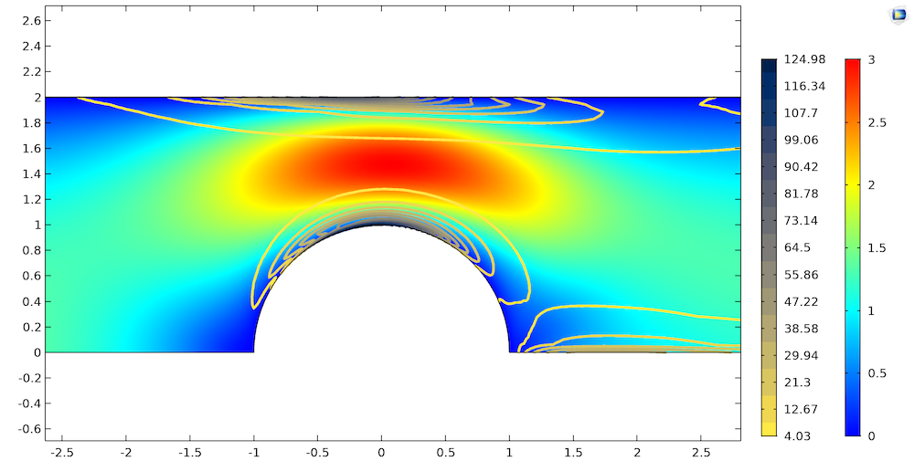
Flow field (Rainbow) and T11 stresses (Cividis contour lines) of the Oldroyd-B fluid in the channel.
The results for the Oldroyd-B fluid model are in good agreement with both experimental and simulation results that have been published in literature, validating the use of COMSOL Multiphysics and the CFD Module for the numerical simulation of viscoelastic flow.
Next Steps
Try solving the Oldroyd-B model yourself: Click the button below, which will take you to the Application Gallery. From there, you can download a step-by-step guide and the MPH-file.
Learn more about the features and functionality available for simulating fluid flow with the CFD Module.


Comments (3)
Austin Zhang
September 14, 2018Hi, could this model used for the case Weissenberg Number bigger than 1?
Sina Ghalambor
December 1, 2018Hi,it is great, and thank you for the nice description. I went through the equations and the COMSOL file.
My question is how the T11, T22, … affect the spf physic? How the calculated values of T11, T12 and T22 affect the velocities in spf physic?
Angshuman Neogi
August 11, 2022Hi,could you provide the same with viscoelastic+2phase flow