Wave Optics Module
New App: Plasmonic Wire Grating Analyzer
This application computes coefficients of refraction, specular reflection, and first-order diffraction as functions of the angle of incidence for a wire grating on a dielectric substrate. The incident angle of a plane wave is swept from the normal angle to the grazing angle on the grating structure. The application also shows the electric field magnitude for multiple grating periods for a selected angle of incidence.
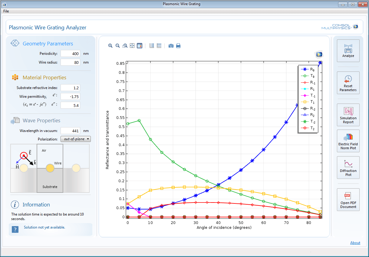 An app that computes diffraction efficiencies for the transmitted and reflected waves (m = 0) and the first and second diffraction orders (m = ±1 and ±2) as functions of the angle of incidence for a wire grating on a dielectric substrate. The wavelength, polarization, material properties, wave periodicity, and radius can be changed.
An app that computes diffraction efficiencies for the transmitted and reflected waves (m = 0) and the first and second diffraction orders (m = ±1 and ±2) as functions of the angle of incidence for a wire grating on a dielectric substrate. The wavelength, polarization, material properties, wave periodicity, and radius can be changed.
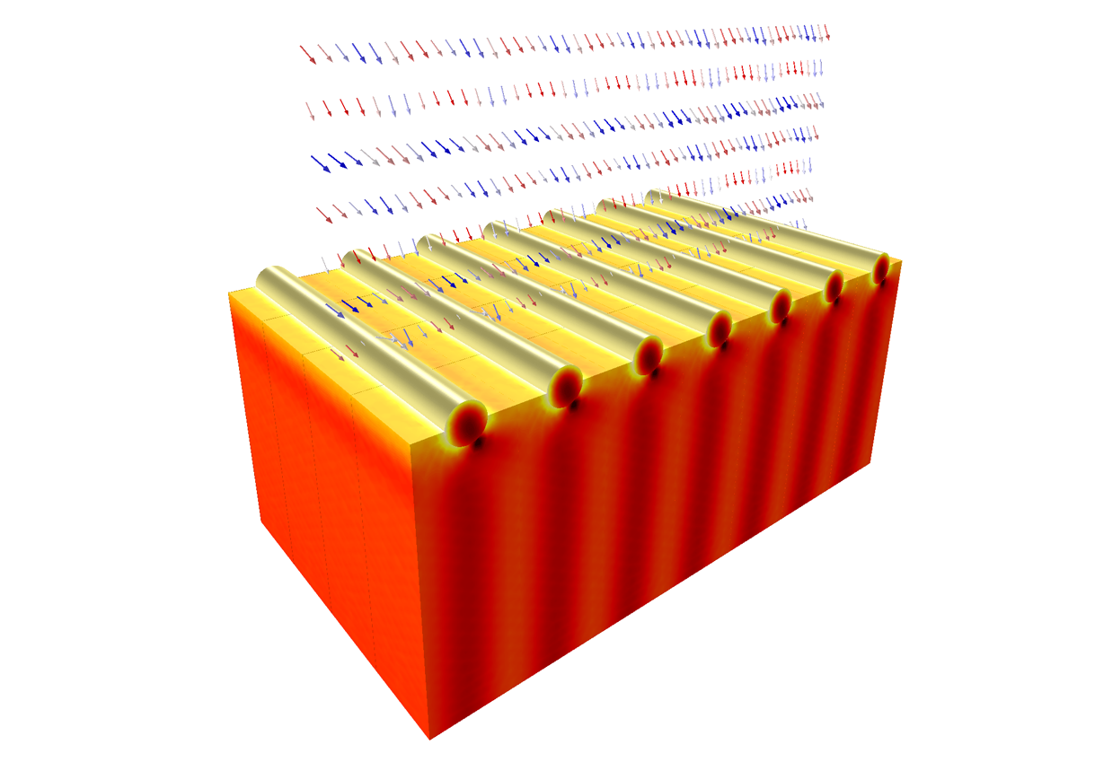 Conceptual image of the underlying model for the app. Shown is the norm of the electric field.
Conceptual image of the underlying model for the app. Shown is the norm of the electric field.
Postprocessing Wave Vector Variable for Periodic Port and Diffraction Order Port
Postprocessing variables are added for the wave vectors for the incident wave and the various diffraction orders (including the reflected wave). These variables can be used in arrow plots for visualization of the various diffraction orders from gratings and other periodic structures.
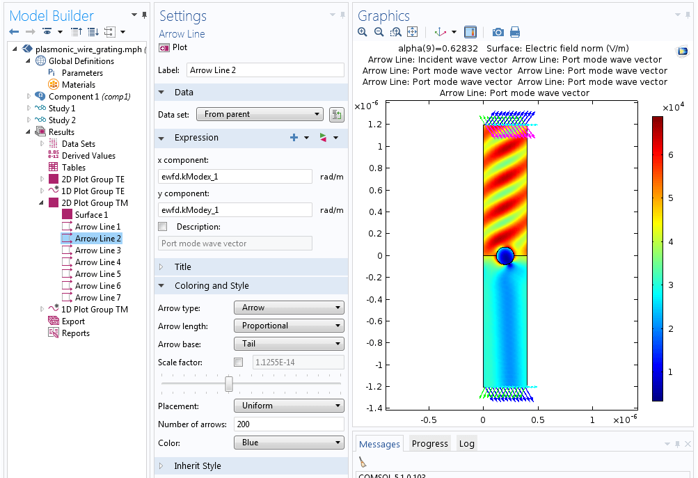 Arrow plot showing the various diffraction orders of a plasmonic wire grating.
Arrow plot showing the various diffraction orders of a plasmonic wire grating.
Scattering Boundary Condition in 2D Axisymmetry Now Handles Incident and Scattered Plane Waves
The Scattering boundary condition for 2D axisymmetric models now includes a plane wave option for the scattered wave type. This means that you can now set up the Scattering boundary condition to absorb a wave propagating along a coaxial waveguide, as shown in the example below. Furthermore, it is also possible to enter the field of an incident wave propagating along the symmetry axis. This is useful for exciting and absorbing waves propagating along coaxial waveguides if you do not want to use Lumped Port excitation. It is also useful for propagating Gaussian beams in free space.
 The picture above shows the setting for the Scattering boundary condition, when exciting an incident wave propagating along a coaxial waveguide.
The picture above shows the setting for the Scattering boundary condition, when exciting an incident wave propagating along a coaxial waveguide.
New Constitutive Relation to the Frequency Domain Interface: Loss Tangent; Loss Angle; and Loss Tangent, Dissipation Factor
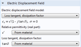
The old loss tangent model has been renamed Loss tangent, loss angle. A new electric displacement field model called Loss tangent, dissipation factor has been added from which it is possible to enter a value directly for the material dissipation factor.
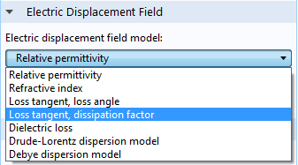 The new Loss tangent, loss angle and Loss tangent, dissipation factor models.
The new Loss tangent, loss angle and Loss tangent, dissipation factor models.
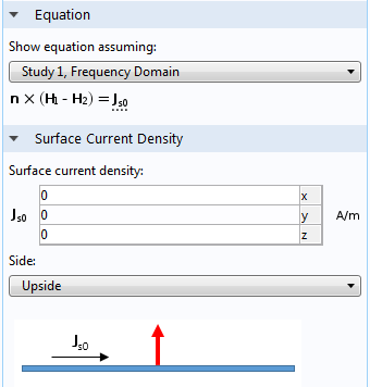
Surface Current Density on Transition Boundary Condition
This subfeature for the Transition boundary condition is a one-sided surface current source that is useful for EMI/EMC applications. It models an imposed current flowing along one side of a thin conductive sheet.
Time-Domain Modeling of Dispersive Drude-Lorentz Media
Plasmonic hole arrays have attracted great interest throughout the last decade since the discovery of extraordinary transmission through sub-wavelength hole arrays. The classical Bethe theory predicts that transmittance through a sub-wavelength circular hole in a PEC screen scales as (d/lambda)^4. Yet, transmission through holes in realistic metallic films can exceed 50% and even approach 100%. This phenomenon is attributed to surface plasmon polaritons, which can tunnel EM energy through the hole even if it is very sub-wavelength. This model is intended as a tutorial that shows how to model the full time-dependent wave equation in dispersive media such as plasmas and semiconductors (and any linear medium describable by a sum of Drude-Lorentz resonant terms).
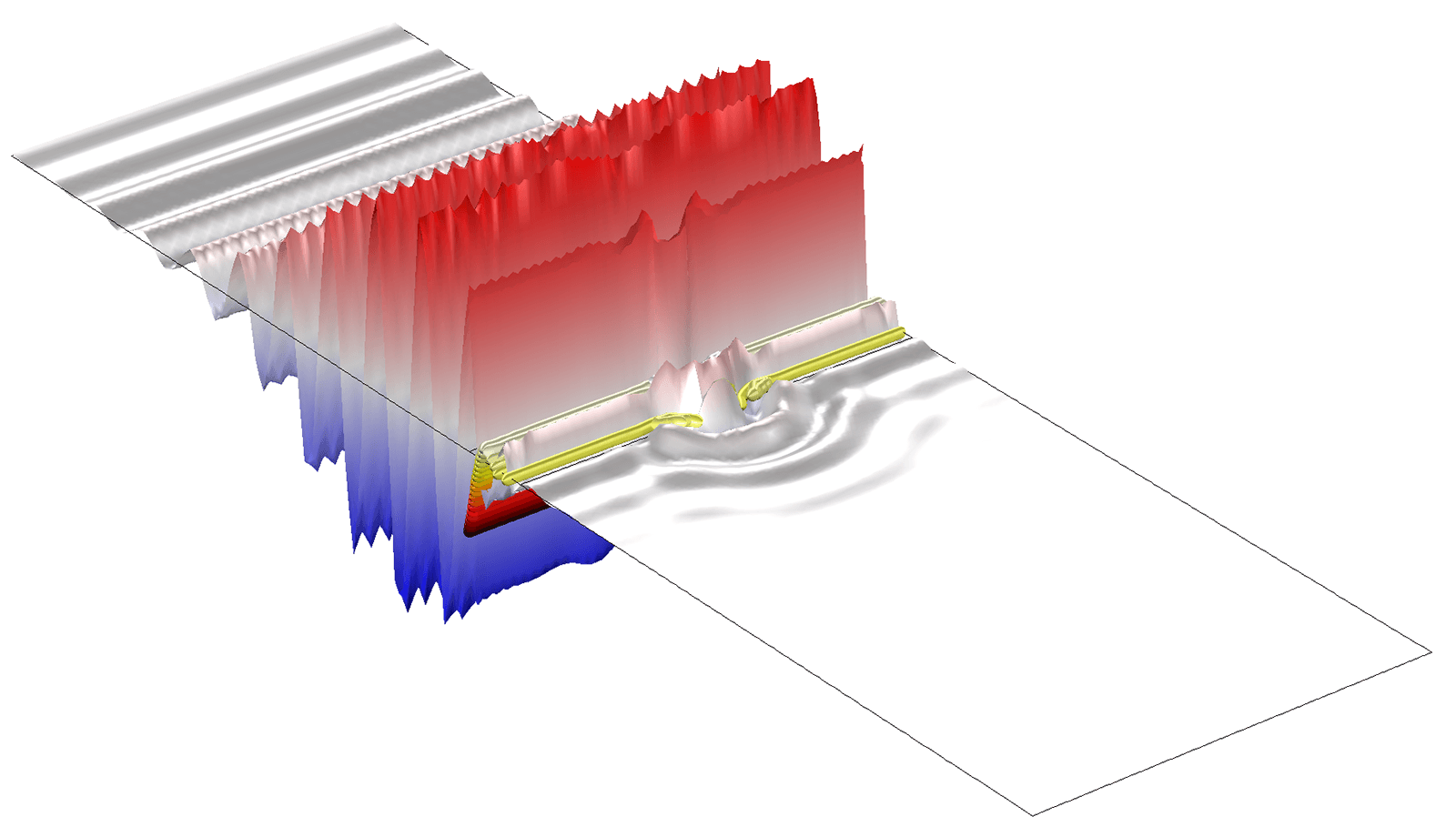 An electromagnetic wave pulse propagates through a sub-wavelength hole in a dispersive dielectric slab.
An electromagnetic wave pulse propagates through a sub-wavelength hole in a dispersive dielectric slab.
Wavelength Domain Study Type Added
With the Wavelength domain study step, you can now sweep the vacuum wavelength, instead of sweeping the frequency as is done for the Frequency domain study. The Wavelength domain study creates the variables root.lambda0 and phys.lambda0 (where "phys" is the tag of the physics interface), which represent the vacuum wavelength. The frequency is still the driving parameter for the Electromagnetic Waves, Frequency Domain and the Electromagnetic Waves, Beam Envelopes interfaces, but now root.freq is defined as c_const/root.lambda0. When plotting global parameters, like the S-parameters against the sweep parameter, the wavelength automatically appears on the x-axis.
The following models now use the Wavelength domain study, instead of the Frequency domain study: scattering _ nanosphere, plasmonic _ wire _ grating, scatterer _ on _ substrate, hexagonal _ grating, and self _ focusing.
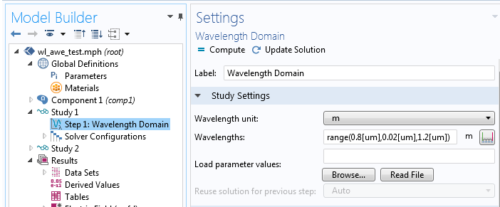 Settings window for the Wavelength domain study.
Settings window for the Wavelength domain study.
Hexagonal Periodic Structures
Hexagonal periodic structures are now correctly analyzed using periodic ports. You only need to specify the incident wave direction to the sides of the hexagonal cell and all periodic boundary conditions will be applied appropriately. Periodic ports have also been improved to handle partitioned port boundaries.
 Simulation of a grating using the new Hexagonal periodic structures.
Simulation of a grating using the new Hexagonal periodic structures.
Time-Domain Modeling of Dispersive Drude-Lorentz Media
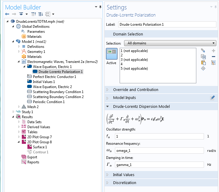
For the Electromagnetic Waves, Transient interface, you can now use the Drude-Lorentz dispersion model from the available Electric displacement field models. The Drude-Lorentz polarization feature can now be added as subfeatures to the wave equation feature. The Drude-Lorentz polarization feature adds the following equation to the desired domains:
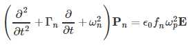
This equation will be solved together with the time-dependent wave equation for the magnetic vector potential.
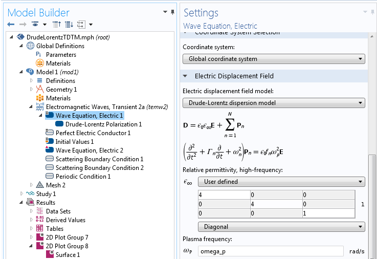 Screenshot of the selection of the Drude-Lorentz dispersion model in the Wave Equation, Electric settings.
Screenshot of the selection of the Drude-Lorentz dispersion model in the Wave Equation, Electric settings.
Field Continuity Feature Added to the Unidirectional Beam Envelopes Interface
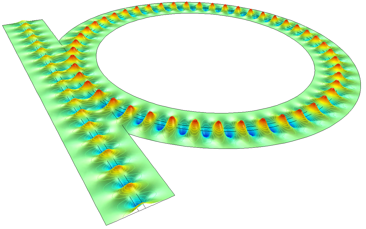
To model the ring resonator in the picture below, you can use the unidirectional formulation of the Electromagnetic Waves, Beam Envelopes interface. To handle structures such as a ring resonator, you must enter a phase function for the wave that increases as the wave propagates clockwise in the ring (assuming that the wave is propagating in the straight waveguide from the bottom to the top). To close the loop, you must introduce, somewhere, a jump in the phase function. In the model shown in the image, the jump in phase is introduced at the interior boundary between the straight and the ring waveguide. The tangential components of the electric and magnetic fields are enforced to be continuous at the boundary with the new Field Continuity boundary condition.
This boundary condition is only available for unidirectional propagation and on interior boundaries. It is normally hidden, but becomes available if Advanced Physics Options is selected in the Show menu in the Model Builder toolbar.
 Simulation of an Optical ring resonator notch filter using the new Field Continuity feature.
Simulation of an Optical ring resonator notch filter using the new Field Continuity feature.
New Optical Materials Database
The new Optical Materials Database will be available for the Ray Optics and the Wave Optics modules. It contains data for a large number of materials for the dispersion of the real and imaginary parts of the refractive index. Among the materials are a large number of glasses used for lenses, semiconductor materials, and other areas. The following models now use the Optical Materials Database: scattering _ nanosphere, plasmonic _ wire _ grating, and scatterer _ on _ substrate.
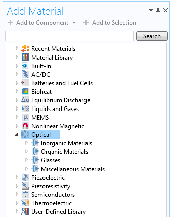 Screenshot of the Optical Materials Database with over 1400 materials
Screenshot of the Optical Materials Database with over 1400 materials
S-parameters Set to Zero for Evanescent Modes
For port modes that are not propagating (evanescent), the S-parameters are now automatically set to be zero. Thus, you do not need to add logical expressions that nullify the S-parameters for frequencies/angles where the corresponding wave is evanescent. This simplifies the use of the S-parameters in postprocessing.
New Tutorial: Hexagonal Grating
A plane wave is incident on a reflecting hexagonal grating. The grating cell consists of a protruding semisphere. The scattering coefficients for the different diffraction orders are calculated for several different wavelengths.
 The norm of the electric field (color plot) and the time-averaged Poynting vector (arrow plot) of part of a hexagonal grating.
The norm of the electric field (color plot) and the time-averaged Poynting vector (arrow plot) of part of a hexagonal grating.
New Tutorial: Optical Ring Resonator Notch Filter
This model calculates the spectral properties of an optical ring resonator. The model demonstrates how to use the Field Continuity boundary condition at boundaries, where there is a jump in the predefined phase approximation.
 This picture shows the out-of-plane component of the electric field in the optical ring resonator for a wavelength close to resonance.
This picture shows the out-of-plane component of the electric field in the optical ring resonator for a wavelength close to resonance.