Modeling Step Transitions
You may want to define loads, material properties, or boundary conditions that vary abruptly with respect to the solution or with respect to time. However, this can lead to a solution that is discontinuous in space and/or time, which can be difficult to solve. One solution is to use smoothed step functions, which we will demonstrate in this article.
Defining and Using Smoothed Step Functions
There are several built-in functions that include a smoothing option. This smoothing can be either first-order or second-order continuous. Second-order continuous is the default and is appropriate in most cases. The functions that include smoothing are: Ramp; Rectangle; Step; Triangle; Waveform (of type Sawtooth, Square, or Rectangle); and Piecewise. The Settings windows for the Step and Piecewise functions, as well as a visualization of the resultant smoothed functions, are shown in the screenshots below.
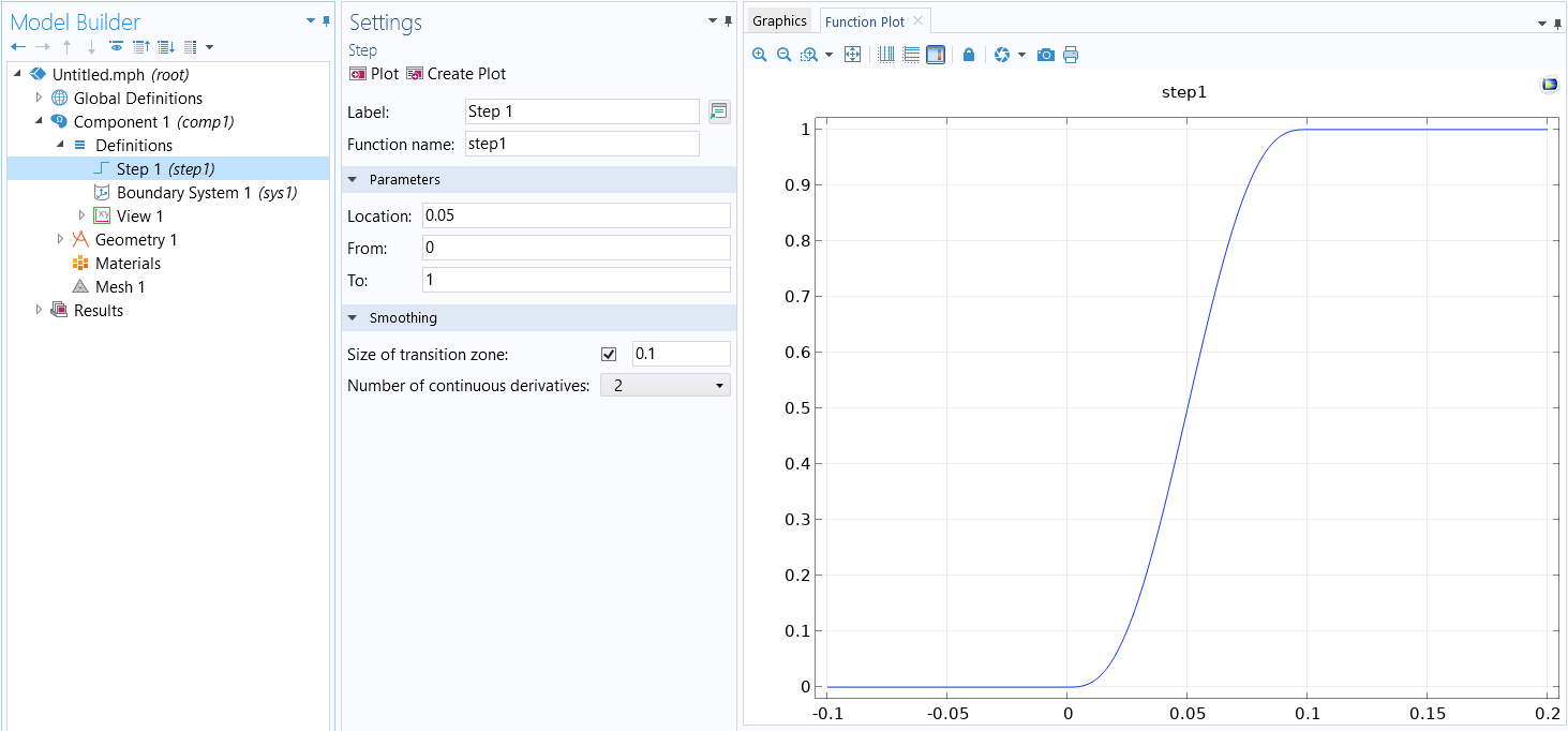 A screenshot of the Model Builder with the Step function Settings window open and the Parameters and Smoothing sections expanded, as well as a smoothed step function shown in the Graphics window.
The Settings window for the Step function and the resultant smoothed step function.
A screenshot of the Model Builder with the Step function Settings window open and the Parameters and Smoothing sections expanded, as well as a smoothed step function shown in the Graphics window.
The Settings window for the Step function and the resultant smoothed step function.
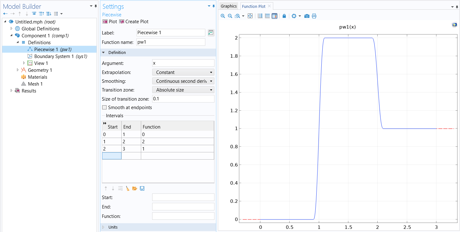 A screenshot of the Model Builder with the Piecewise function Settings window open and the Definition section expanded, as well as a smoothed piecewise function shown in the Graphics window.
The Settings window for the Piecewise function and the resultant smoothed piecewise function.
A screenshot of the Model Builder with the Piecewise function Settings window open and the Definition section expanded, as well as a smoothed piecewise function shown in the Graphics window.
The Settings window for the Piecewise function and the resultant smoothed piecewise function.
Smoothed step functions, as well as other functions, can be defined at the global level under the Global Definitions node, locally within the Definitions node of a Component within the model, or within the Materials node property definitions, depending upon the desired scope of the function.
After defining the function, you can call out its use from within your model for other settings. In the simple, transient fluid flow model included here, we demonstrate using a smoothed step function to ramp up a boundary condition, the inlet velocity, so that it is consistent with the initial values.
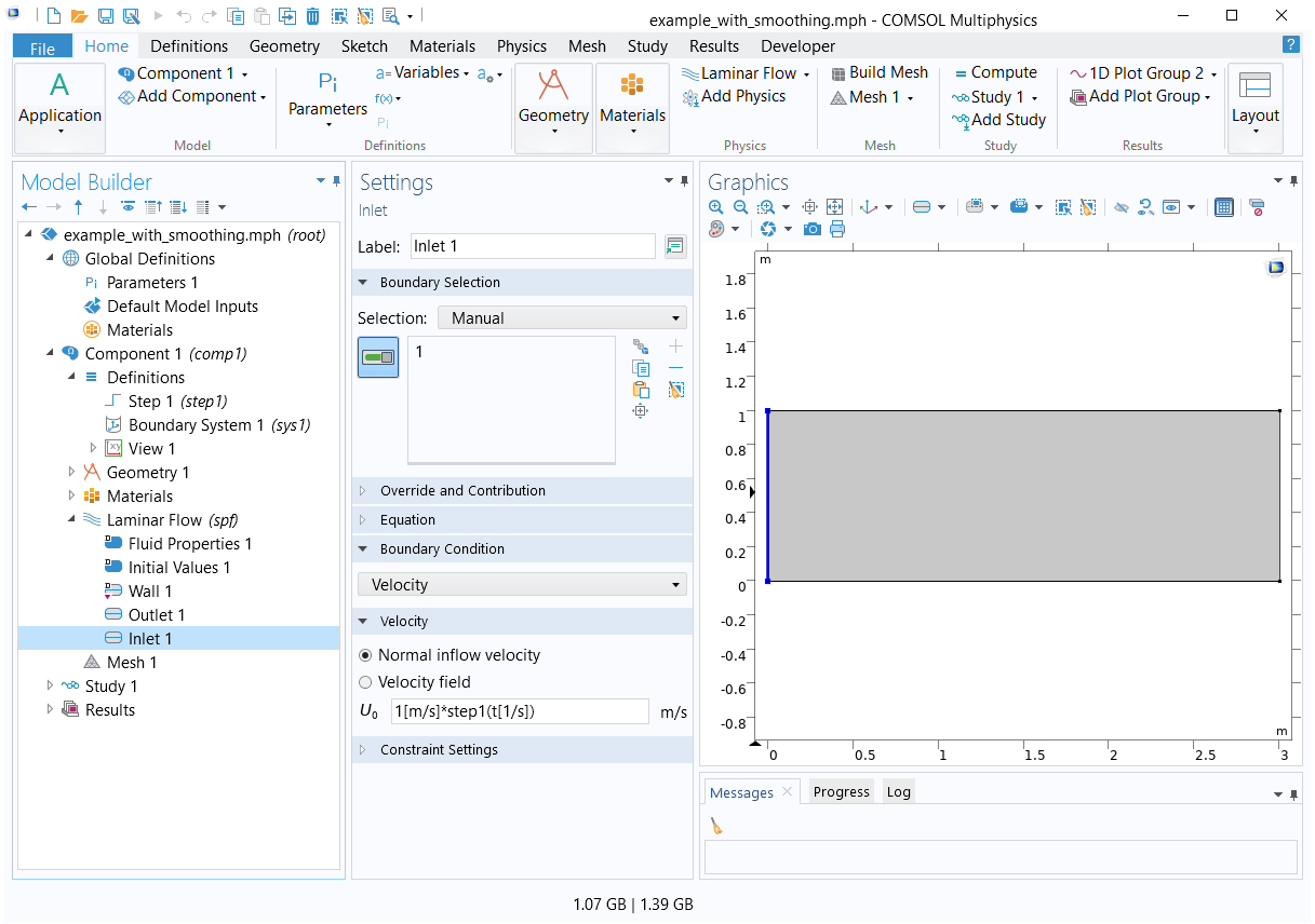 A screenshot of the Inlet Settings window, with the Boundary Condition section expanded to show the velocity settings for a fluid flow model.
Settings for the velocity at the inlet for the example fluid flow model attached.
A screenshot of the Inlet Settings window, with the Boundary Condition section expanded to show the velocity settings for a fluid flow model.
Settings for the velocity at the inlet for the example fluid flow model attached.
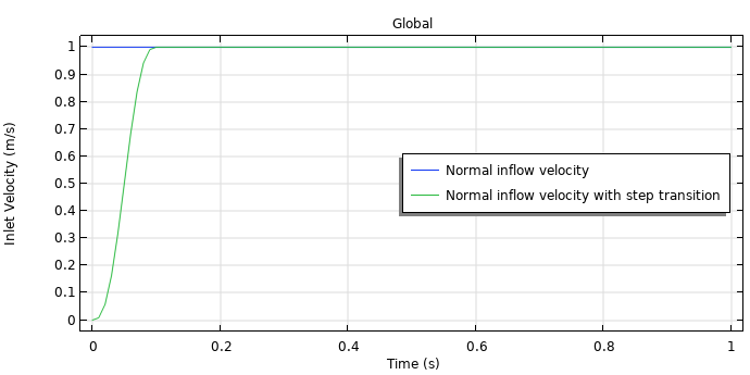
Plot of the inlet velocity for the example fluid flow model attached, both with smoothing (green) and without smoothing (blue), provided through defining and using a Step function. For problems like these, you will need to choose a timespan for the smoothing that is realistic for the problem at hand.
There are several tutorial models in the Application Libraries that utilize Step functions to model a step transition. The table below lists some of these models and includes a brief description for the application of the smoothed step function, which you can look further into for details on the implementation and logic employed.
| Model | Step Transition Application | |
|---|---|---|
| 1 | Flow Past a Cylinder | Ramp up the inflow velocity |
| 2 | Micromixer | Impose a concentration gradient |
| 3 | Internal Short Circuit in a Lithium-Ion Battery | Ramp up the electrical conductivity of the penetrating filament |
| 4 | Polymer Electrolyte Membrane Electrolyzer | Improve convergence when solving |
| 5 | Thin Layer Chronoamperometry | Step the concentration from initial conditions to zero |
| 6 | Heat Conduction in a Finite Slab | Avoid jump between initial conditions and boundary conditions |
| 7 | Phase Change | Avoid discontinuity between start time and boundary condition |
| 8 | Pull-In of an RF MEMS Switch | Represent the dielectric constant within the domain |
| 9 | Electroosmotic Micromixer | Impose a step in the concentration |
| 10 | Wicking in a Paper Strip | Step the capillary pressure to zero when soaked with water |
| 11 | Two-Mirror Laser Cavity | Plot the model's analytical result versus simulation result for comparison |
| 12 | Laser Cavity with a Thin Lens | Plot the model's analytical result versus simulation result for comparison |
Other Resolutions
For instantaneous switching in time-dependent models, there is also a resolution apart from the one discussed in this article that you can utilize. You can use the Events interface, as explained here, for solving model cases such as these.
Submit feedback about this page or contact support here.