
Have you ever wondered how some ice cream, pudding, and candies get their outstanding, vivid yellow color? Vitamin B2 is used as a food additive to dye these products. In industry, vitamin B2 is mainly produced by a biotechnological process. A lot of products in our day-to-day life include ingredients produced by such processes, including bioethanol (fuel), citric acid (a cleaning agent), and vitamin C (a food additive). To fabricate these chemical compounds, we use the metabolic pathways of microorganisms consisting of biochemical reactions. Let’s see how modeling can help us understand the dynamics of metabolic pathways.

Certain candies get their vivid yellow color from the food additive vitamin B2. Image by Evan-Amos — Own work. Licensed under CC BY-SA 3.0, via Wikimedia Commons.
Introduction to Metabolic Reaction Networks
To understand and optimize biotechnological processes and the microorganisms involved, the fields of systems biology and metabolic engineering use mathematical models. These models are often based on the assumption that the microbial cells, with their coupled biochemical reactions inside, can be seen as perfectly mixed systems. The models used for such systems are those of the ideal tank reactor. The term metabolic reaction network describes biochemical reaction systems with multitude coupled reactions.
In the Chemical Reaction Engineering Module, an add-on to the COMSOL Multiphysics® software, the Reaction Engineering interface offers predefined functionality to model ideal tank reactors. Besides the predefined functionality for modeling chemical kinetics based on the mass action law, researchers and engineers can define their own kinetic expressions using the powerful functionality for equation-based modeling. Once defined, the chemistry, kinetics, and thermodynamics for an ideal tank reactor model can be used to automatically generate full space-dependent models with transport and reactions.
In this blog post, we will use the Reaction Engineering interface and the equation-based modeling functionality to set up a model for the glycolysis metabolic pathway of yeast, which is central for living cells. The model can help us understand experimentally observed oscillation dynamics and stems from the paper by Wolf et al. (Ref. 1).
Modeling Intracellular Dynamics in Yeast
The glycolysis metabolic pathway is a central reaction sequence in almost all organisms. This pathway converts monosaccharides (simple sugar), such as glucose, to metabolic intermediates. During this conversion process, the energy stored in sugar is released and the energy carrier molecules ATP (adenosine triphosphate) and NADH (reduced nicotinamide adenine dinucleotide) are formed. These high-energy molecules provide energy for other processes in the cell. In addition, the metabolic intermediates produced by glycolysis are utilized in other metabolic pathways to, e.g., synthesize building blocks for cell material such as fatty or amino acids.
Considering this, it is clear that the glycolysis metabolic pathway is interconnected with other metabolic pathways, forming a large metabolic reaction network. Complex reaction schemes can give rise to nontrivial system dynamics.
For yeast, it is known that under certain conditions, the concentrations of metabolic compounds of the glycolysis metabolic pathway oscillate. These oscillations can propagate within and between yeast cells. This phenomenon was investigated by the researchers Wolf et al. They developed a minimum model for the glycolysis metabolic pathway in yeast cells. The model includes lumped reactions for the following processes:
- Glycolytic pathway
- Production of glycerol
- Fermentation to ethanol
- Exchange of acetaldehyde between the cells
- Trapping of acetaldehyde by cyanide
This minimum model reflects the essence of experimentally observed oscillations. Let’s see what this model looks like and what assumptions are made.
A basis reaction scheme for the examined metabolic pathway, including fluxes, is shown below.
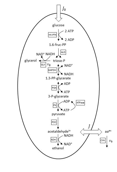
Basis reaction scheme for the anaerobic glycolytic pathway. Abbreviations for the enzyme reactions are marked with boxes. Scheme and abbreviations are adapted from Wolf et al. (Ref. 1).
Under the considered conditions, the respiration is absent and therefore neglected in the reaction scheme. As a consequence, ethanol is the main end product of glycolysis here. Glucose is transported via an extracellular flux (J_0) into the cell. The concentrations of ethanol and glycerol are fixed in the model because equilibration between the intracellular and large extracellular pool is assumed. The considered minor side fluxes are:
- Exchange flux between the cell’s internal and external medium acetaldehyde (J)
- Glycerol formation flux (v_8)
- Extracellular degradation of acetaldehyde due to cyanide (v_9)
The cell membrane is supposed as impermeable for the other metabolites beside glucose, acetaldehyde, and ethanol.
Furthermore, the derived nine-variable metabolite model is depicted below.
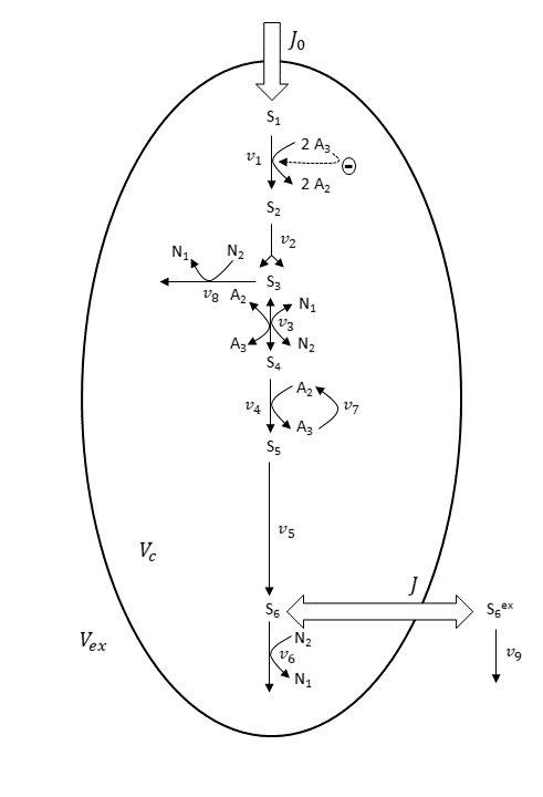
Scheme for the nine-variable metabolite concentration model. Scheme and abbreviations are adapted from Wolf et al. (Ref. 1).
In the nine-variable model, the majority of reactions are assumed irreversible. The enzyme reactions of GAPDH and PGK, shown in the first basis reaction scheme, are combined to one reversible reaction (v_3), shown in the nine-variable model scheme.
Mass-action-law-based rate expressions are used to describe all enzyme reactions. For the HK–PFK reaction (v_1), regulatory properties are considered. This means the reaction is inhibited by ATP (A_3). The intracellular pools of the adenine nucleotides ADP (A_2) and ATP (A_3), and of the nicotinamide adenine dinucleotides NAD+ (N_1) and NADH (N_2), are assumed to be constant.
Under the assumption of perfectly mixed solutions inside and outside the cell, Wolf et al. (Ref. 1) used a system of differential algebraic equations (DAEs) to describe the model. More detailed information about initial conditions, rate constants, and more can be found in the paper of Wolf et al. (Ref. 1).
In COMSOL Multiphysics, the Reaction Engineering interface is the suitable tool to create a model for the system described above. By just typing in the reactions stated in the last reaction scheme and defining the kinetics by mainly using predefined mass action law kinetics, you can easily create the model. This follows the principle of “what you see is what you get”.
By just typing in the reactions of the reaction scheme in the Reaction Engineering interface, the core of the model is quickly defined.
As an example for a special rate expression manually defined in the model, you can state the rate expression for the HK–PFK reaction (Reaction 1):
(1)
(2)
Here, the inhibition of the enzyme reaction by ATP (A_3) is described by f(A_3). We will see below how this will be implemented in the COMSOL® software.
Finally, for the COMSOL Multiphysics model, we use the predefined functionality for a perfectly mixed batch reactor. This seems, at first glance, to be opposed to the reaction scheme with its fluxes through the cell membrane. Intuitively, a continuous stirred-tank reactor (CSTR) comes into mind. However, since we have no control of the outflux in the above-described model, a batch reactor model with an extra manually defined source for flux J_0 is appropriate.
Let’s see how the model building process is done in the COMSOL® software.
Using the Reaction Engineering Interface to Simulate Metabolite Dynamics
To define the above-described model and compute the time-dependent metabolite concentrations, we can create a 0D model with the Reaction Engineering interface and use a time-dependent study in COMSOL Multiphysics.
In the Model Wizard, we can select 0D for the space dimension:

To create a COMSOL Multiphysics model for an ideal batch reactor, select 0D for the space dimension.
In the Select Physics step, we select the Reaction Engineering interface under the Chemical Species Transport branch:

Select the Reaction Engineering interface in the Select Physics step.
In the last step of the Model Wizard, choose Time Dependent for the study type:

Select a Time Dependent study.
Once this is done, we can stay with the default reactor type Batch, constant volume of the Reaction Engineering interface. How we modify this with an Additional Source for J_0 is described below.
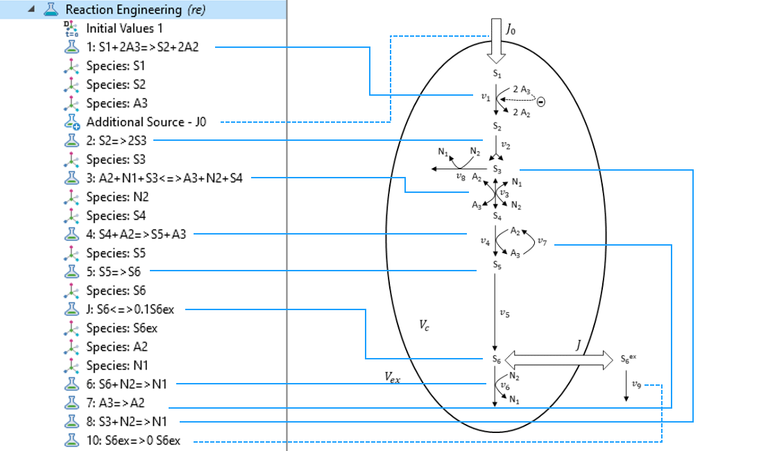
Next, we can use the Reaction functionality under the Reaction Engineering tab to define every reaction considered in the model. In the Formula field of the Reaction Formula section, we type in the stoichiometry of the considered reaction. For example, for defining the stoichiometry of an irreversible reaction, we can use => for the reaction arrow.
If a user-defined expression other than a typical mass action law for the reaction rate is needed, we choose User Defined in the Reaction Rate section and type in the corresponding expression. Here, parameters, as well as user-defined and built-in variables, can be used to define the expression for the reaction rate. By using the Reaction functionality, the COMSOL® software automatically creates Species nodes for the metabolites involved in the defined reactions. This means that the balance equations for the metabolites are automatically generated.
For instance, for defining Eq. 1, we use the built-in concentration variables re.c_S1 and re.c_A3 of the Reaction Engineering interface for the metabolites S_1 and A_3, respectively. k1 is a defined parameter in the Parameters node and f_A3 is a defined variable for Eq. 2 in the Variables node.

Use the Reaction functionality in the Reaction Engineering tab in the toolbar to define all relevant reactions of the model. The stoichiometry is defined in the Formula input field of the Reaction Formula section. In the Reaction Rate section, we can choose User defined to define an individual rate expression.
Next, the Additional Source feature is used to add the source term J_0 to the balance equation of metabolite S_1. J0 is a parameter defined in the Parameters node.

Introducing an Additional Source found in the Global section in the toolbar to add the source term J0 to the balance equation of metabolite S_1.
To model the extracellular degradation of acetaldehyde due to cyanide (v_9), we introduce reaction 10 in the model. On the product side of the reaction, a stoichiometric coefficient of 0 for S_6^{ex} is set, since we need to state a product when we want to define a reaction via the Reaction feature. This perfectly defines the rate expression as independent of product concentrations.

A stoichiometric coefficient of 0 for S_6^{ex} on the product side of reaction 10 is used to define v_9 via the Reaction feature. Assuming a mass action law kinetic expression, this gives a rate expression independent of product concentrations and reproduces the reaction scheme.
Finally, after the definition of the model by applying the mentioned features of the Reaction Engineering interface, we can solve the model with the time-dependent study.
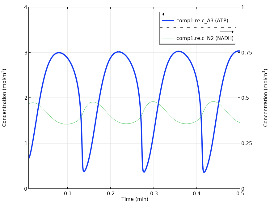
Solving the time-dependent model yields oscillating metabolite concentrations for ATP (A_3) and NADH (N_2).
The graph shown above reproduces the results in Fig. 4. of Wolf et al.’s paper (Ref. 1). The same oscillations in the metabolite concentrations were found.
Concluding Thoughts
In this blog post, we demonstrated how the Reaction Engineering interface of the Chemical Reaction Engineering Module can be used to model metabolic pathways described by differential and algebraic equations. The predefined features in a user-friendly graphical user interface accelerate the model-building process for such tasks. In addition, by using the equation-based modeling capabilities of COMSOL Multiphysics, we can create individual user-defined models. Also, more complex reaction systems can be modeled and analyzed this way.
Next Steps
Try the model discussed here by clicking the button below:
Further Reading
Want to read more about modeling of reaction kinetics? Check out these blog posts:
- Enzyme Kinetics, Michaelis-Menten Mechanism
- A General Introduction to Chemical Kinetics, Arrhenius Law
- Chemical Parameter Estimation Using COMSOL Multiphysics
- Apps for Teaching Mathematical Modeling of Tubular Reactors
Reference
- J. Wolf et al., “Transduction of Intracellular and Intercellular Dynamics in Yeast Glycolytic Oscillations”, Biophys. J., vol. 78, pp. 1145–1153, 2000, (https://www.sciencedirect.com/science/article/pii/S0006349500766720).


Comments (0)