
The Tubular Reactor application is a tool where students can model a nonideal tubular reactor, including radial and axial variations in temperature and composition, and investigate the impact of different operating conditions. It also exemplifies how teachers can build tailored interfaces for problems that challenge the students’ imagination. The model and exercise are originally described in Scott Fogler’s book Elements of Chemical Reaction Engineering. I wish I had access to this type of tool when I was a student!
Apps Simplify Teaching and Learning Mathematical Modeling Concepts
I still remember the calculus classes at engineering school where we first encountered partial differential equations. Despite the teacher’s efforts in trying to exemplify diffusion with the distance and the time it takes for a shark to detect your blood in the water if you cut yourself while diving, the rest of the course was mostly overshadowed by theorems. Theorems that could prove existence and uniqueness, for relatively simple problems, and by techniques such as variable separation and conformal mapping.
Apart from math theory and solving techniques, I realize now that what we really needed, in order to understand mathematical models, was to study the solution to the model equations and investigate this for different assumptions and conditions.
The Tubular Reactor with Jacket application in the COMSOL Multiphysics® software version 5.0 gives students the possibility to go from a mathematical model of a nonideal tubular reactor straight to the solution of the corresponding numerical model. The model is taken from an exercise in Scott Fogler’s book Elements of Chemical Reaction Engineering, which is one of the most popular books in undergraduate and graduate courses in chemical reaction engineering.
")
Figure 1. The Tubular Reactor application’s user interface together with a possible workflow, Steps 1 to 5.
Value to the Student
The mathematical model consists of an energy balance and a material balance described in an axisymmetric coordinate system. As a student, you can change the activation energy of the reaction, the thermal conductivity, and the heat of reaction in the reactor (see Step 2 in the figure above). The resulting solution gives the axial and radial conversion and temperature profiles in the reactor. For some data, the results from the simulation are not obvious, which means that the interpretation of the model results also becomes a problem-solving exercise.
Value to the Teacher
The Tubular Reactor app can be accessed by a teacher in the Application Builder. As a teacher, you can investigate how to include model and application documentation in an application’s user interface. You can also learn how to include user interface commands that allow the students to generate a report from each simulation. In addition, the application accessed in the Application Builder also shows you how to create menu bars, ribbons, ribbon tabs, form collections, and forms in an application’s user interface and how to link these user interface components with settings and results in the underlying embedded model.
The Tubular Reactor Application
The different steps in the exercise for the tubular reactor problem are reflected in the ribbon on Windows® operating systems or in the main toolbar on Linux® operating systems and Mac OS in the application’s user interface.
The natural first step is to read the documentation (see Step 1 in Figure 1 above). The students can then change the activation energy and the heat of reaction, as well as the thermal conductivity in the reactor in Step 2.
The third step is to compute the solution to the model equations (Step 3). This makes it possible for the students to analyze the solution in four different plots (Step 4): Two surface plots that show the temperature and the conversion of the reactant in the reactor, and two cut line plots that show the temperature and conversion of the reactant in the reactor along three different lines placed at three different z-positions (see Figure 3 further down the page for an example). The four different plots are found under their respective tabs in a so-called form collection.
The last step is to generate a report (Step 5) that documents the model and the results from the simulation. In this case, the output is in Microsoft® Word® format, but you may also generate HTML reports.
For the teacher, the application builder tree and the member form preview in the Application Builder reveal the structure of the app (see Figure 2 below). The Main Window node (labeled 1 in the screenshot below) contains the child nodes that describe the file menu (2) and the ribbon (3). In Linux® operating systems, the ribbon is shown as a toolbar. It also contains a reference to the main form. The Form node (4) contains five forms in this case: One form that describes the main form and four forms that describe the different members in the graphics form collection. These four graphics form members correspond to the four plots mentioned above.
")
Figure 2. The Application Builder user interface that includes the application builder tree to the left and the preview of the included forms to the right. In between is the settings window for each selected form, declaration, method, library, or model nodes.
The text input widgets for the activation energy, the thermal conductivity, and the heat of reaction (5) are linked to the corresponding parameters in the embedded model. The range of values is also limited in order to provide a safe input range that does not produce garbage.
The Declarations node (6) includes the declaration of variables that are not defined in the embedded model. For instance, you can declare a string variable that displays a message in the user interface when the app is run based on a selection by the user. In this example, a string variable is created to show if the simulation results are updated or not (i.e., if the student changes the activation energy without re-solving the model equation, a string variable displayed in the graphics window is set to “*Not Updated”).
The application further contains a set of methods (7) that correspond to loading the model documentation, computing the results in a simulation, and generating the report. These methods are linked to the corresponding menus in the ribbon or in the main menu. The methods are graphically generated, but can then be edited manually using the method editor for further flexibility.
The Library node (8) contains files that are embedded in the application. In this example, we have a PDF-file that contains the application’s documentation linked to the corresponding ribbon menus.
The Tubular Reactor Model
The process described by the model is that for the exothermic reaction of propylene oxide with water to form propylene glycol. This reaction takes place in a tubular reactor equipped with a cooling jacket in order to avoid explosion (see the figure in the “Model Results” section below).
The reaction takes place in the liquid phase and in the presence of a solvent. The density of the reactor solution is therefore assumed to vary to a negligible extent despite variations in composition and temperature. Under these assumptions, it is possible to define a fully developed velocity profile along the radius of the reactor.
The model equations describe the conservation of material and energy. The dependent variables are the concentration, c, and the temperature, T, in the reactor. The material and energy equations are defined along two independent variables: the variable for the radial direction, r, and along the axial direction, z. These equations form a system of two coupled partial differential equations (PDE), along r and z.
The boundary conditions define the concentration and temperature at the inlet of the reactor. At the outlet, the outwards flux of material and energy is dominated by advection and is described accordingly. At the reactor wall, the heat flux is proportional to the temperature difference between the reactor and the cooling jacket.
(1)
\nabla \cdot \left( { – D\nabla c} \right) + \nabla c \cdot {\bf{u}} + {k_f}c = 0\\
c = {c_0}\quad at\;inlet;\quad \left( {\left( { – D\nabla c} \right) + c{\bf{u}}} \right) \cdot {\bf{n}} = c{\bf{u}} \cdot {\bf{n}}\quad at\;outlet\\
\\
\nabla \cdot \left( { – k\nabla T} \right) + \rho {C_p}\nabla T \cdot {\bf{u}} + {k_f}c\Delta H = 0\\
T = {T_0}\quad at\;inlet;\quad \left( {\left( { – k\nabla T} \right) + \rho {C_p}T\,{\bf{u}}} \right) \cdot {\bf{n}} = \rho {C_p}T\,{\bf{u}} \cdot {\bf{n}}\quad at\;outlet\\
– k\nabla T \cdot {\bf{n}} = {s_a}h\left( {{T_j} – T} \right)\quad at\;reactor\;walls
\end{array}\]
Model Results
The results from the simulation are quite interesting. For example, the conversion profiles along the radial cut lines display a minimum and a maximum, as seen in Figure 3 below. In Fogler’s book, one of the tasks for the student is to explain these profiles.
Here, we can reveal that the profile is explained by the combination of the exothermic reaction, the advective term, and the cooling from the jacket.
In the middle of the reactor, the large flow velocity reduces the conversion, since the reactants reach far into the reactor before they react. This is labeled 1 in Figure 3.
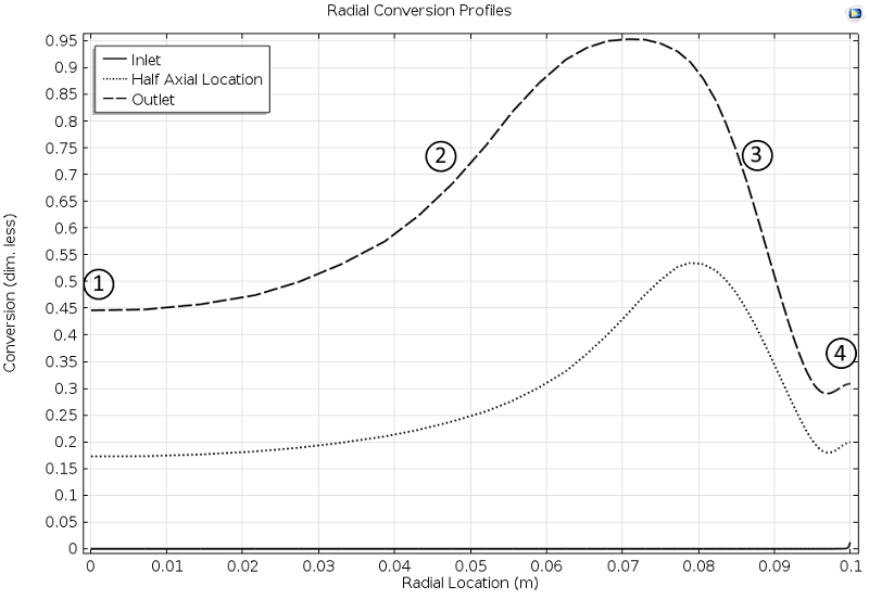
Figure 3. Cut lines plot of the conversion in the reactor along the radial direction at different axial positions: Inlet, half axial location, and outlet.
Closer to the wall, the flow rate decreases and the conversion then increases, since the temperature is still relatively high far from the jacket wall, which also gives a high reaction rate (2).
However, as we get even closer to the wall, the conversion starts to decrease due to the cooling of the jacket, which decreases the reaction rate (3) in the figure above.
At the reactor wall, the cooling is very efficient, which should decrease the conversion even more. However, the conversion increases slightly, since there is no advection of reactants at the wall. In other words, the space time for the volume elements that travel at the wall is very high, since the flow is zero at the wall (4). The reactants are therefore consumed to a larger extent.
Applications in Teaching
The Tubular Reactor example shows how to create a dedicated user interface based on a model — an application — where students can build an intuitive connection between a physical description of a reactor and the implications of this description in the operation of the reactor. An important component in this exercise is that the results are not obvious; the interpretation of the results requires some thinking.
The Application Builder provides a user-friendly tool for the teacher to graphically create application interfaces. It allows teachers to concentrate on the exercise itself rather than investing time in explaining software tools or programming interfaces in the traditional way. They can focus on generating simulation results that trigger thinking.
The students get more challenging and entertaining exercises that focus on the problem, not on the technicalities of running simulation software.
Next Steps
- Intrigued? Learn more about the Application Builder on the 5.0 Release Highlights page.
- Download the Tubular Reactor Jacket app
Microsoft and Windows are either registered trademarks or trademarks of Microsoft Corporation in the United States and/or other countries.
Linux is a registered trademark of Linus Torvalds.
Mac OS is a trademark of Apple Inc., registered in the U.S. and other countries.


Comments (0)