

In electrochemical cell design, you need to consider three current distribution classes in the electrolyte and electrodes. These are called primary, secondary, and tertiary, and refer to different approximations that apply depending on the relative significance of solution resistance, finite electrode kinetics, and mass transport. Here, we provide a general introduction to the concept of current distribution and discuss the topic from a theoretical stand-point.
General Introduction to Current Distribution
An electrochemical cell is characterized by the relation of the current it passes to the voltage across it. The current-voltage relation depends on diverse physical phenomena and is fundamental to performance. In a battery or fuel cell at zero current (equilibrium), a theoretical maximum voltage can be extracted, but we want to draw current in order to extract power.
When current is drawn, there are voltage losses; equally, the current density may not be uniformly distributed on the electrode surfaces. The performance and lifetime of electrochemical cells, such as electroplating cells or batteries, is often improved by a uniform current density distribution.
By contrast, bad design leads to poor performance, such as:
- Substantial losses and shortened lifetime of electrode material at practical operating currents in a battery or fuel cell
- Uneven plating thickness in electroplating
- Unprotected surfaces in a cathodic protection system
Simulating current distribution enables better understanding to avoid such problems.
The current distribution depends on several factors:
- Cell geometry
- Cell operating conditions
- Electrolyte conductivity
- Electrode kinetics (“activation overpotential”)
- Mass transport of the reactants (“concentration overpotential”)
- Mass transport of ions in the electrolyte
Because of this complexity, many applications benefit from suitable simplification when modeling. If one of these factors dominates the cell behavior, the others may not need to be taken into account. As a consequence, successive approximations are introduced by the classifications of primary, secondary, and tertiary current distribution.
Each of the three classes of current distribution is represented in COMSOL Multiphysics by its own interface: Primary, Secondary, and Tertiary Current Distribution. These interfaces are provided in all of the four different application-specific products available for modeling electrochemical cells: the Batteries & Fuel Cells Module, Electrodeposition Module, Corrosion Module, and Electrochemistry Module.
Essential Theory
When modeling an electrochemical cell, you have to solve for the potential and current density in the electrodes and the electrolyte, respectively. You may also have to consider the contributing species concentrations and the involved electrolysis (Faradaic) reactions.
The electrodes in an electrochemical cell are normally metallic conductors and so their current-voltage relation obeys Ohm’s law:
\textbf{i}_s = -\sigma_s\nabla\phi_s\ with conservation of current \nabla\cdot\textbf{i}_s = Q_s
where \textbf{i}_s denotes the current density vector (A/m2) in the electrode, \sigma_s denotes the conductivity (S/m), \phi_s\ the electric potential in the metallic conductor (V), and Q_s denotes a general current source term (A/m3, normally zero).
In the electrolyte, which is an ionic conductor, the net current density can be described using the sum of fluxes of all ions:
where \textbf{i}_l denotes the current density vector (A/m2) in the electrolyte, F denotes the Faraday constant (C/mol), and N_i the flux of species i (mol/(m2·s)) with charge number z_i. The flux of an ion in an ideal electrolyte solution is described by the Nernst-Planck equation and accounts for the flux of solute species by diffusion, migration, and convection in the three respective additive terms:
(1)
where c_i represents the concentration of the ion i (mol/m3), D_i the diffusion coefficient (m2/s), u_{m,i} its mobility (s·mol/kg), \phi_l\ the electrolyte potential, and \textbf{u} the velocity vector (m/s).
On substituting the Nernst-Planck equation into the expression for current density, we find:
(2)
with conservation of current including a general electrolyte current source term Q_l (A/m3):
As well as conservation of current in the electrodes and electrolyte, you also have to consider the interface between the electrode and the electrolyte. Here, the current must also be conserved. Current is transferred between the electrode and electrolyte domains either by an electrochemical reaction, also called electrolysis or Faradaic current, or by dynamic charging or discharging of the charged double layer of ions adjacent to the electrode, also called capacitive or non-Faradaic current.
This general treatment of electrochemical theory is usually too complicated to be practical. By assuming that one or more of the terms in Equation (2) are small, the equations can be simplified and linearized. The three different current distribution classes applied in electrochemical analysis are based on a range of assumptions made to these general equations, depending on the relative influence of the different factors affecting the current distribution as listed above. In the next blog post in the series we’ll discuss the detailed content of these assumptions: going from primary to secondary to tertiary, fewer assumptions are made. Therefore, the complexity increases, but so does the level of detail available from the simulation.
Below you can see the geometry from a modeling example of a wire electrode. This example models the primary, secondary, and tertiary current distributions of an electrochemical cell. In the open volume between the wire and the flat surfaces, electrolyte is allowed to flow. You can think of the electrochemical cell as a unit cell of a larger wire-mesh electrode — a common electrochemical cell set-up in many large-scale industrial processes.
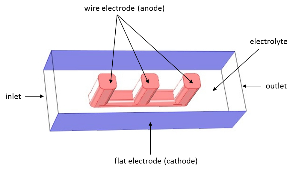
Geometry of the electrochemical cell. Wire electrode (anode) between two flat electrodes (cathodes). Flow inlet to the left, outlet to the right. The top and bottom flat surfaces are inert.
Next Up: Choosing the Right Current Distribution Interface
Now, you might be wondering which of the three current distribution interfaces you should use for your particular electrochemical cell simulations. In an upcoming blog post, we will use the wire electrode example shown here for a comparison of the three current distributions. Stay tuned!


Comments (1)
Andrea Olietti
February 10, 2023Hello, I’m new in the Comsol world, I was reading, from the application file, the wire electrode model builder but I cannot understand why, for the primary current distribution simulation, the phil is texted as (Ecell-Eec,a-Eeq,c)/2. Why is divided by two? Due to the cell’s geometry?
Thank you in advance for the response.