Modeling TEM and Quasi-TEM Transmission Lines
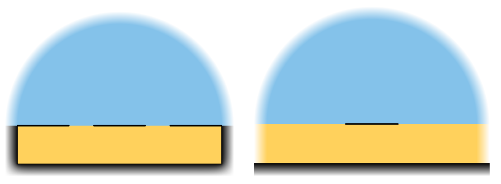
There are four kinds of perfect TEM transmission lines, shown in the image below, including the:
- Coaxial cable
- Line above plane
- Parallel wire
- Parallel plate
All of these consist of two metallic domains, arranged in various configurations. For a true TEM line, the metal is assumed to be an ideal conductor of infinite conductivity, and it is modeled as a Perfect Electric Conductor boundary condition. The space between the PEC boundaries is a homogeneous and lossless dielectric. For the cases of the coaxial cable and parallel plate, the fields are entirely confined between the two conductors. For the other cases, the fields extend infinitely far into the surrounding space, but fall off to zero very quickly. The electric and magnetic fields lie purely in the cross-sectional plane of the line, and the Poynting flux is everywhere parallel to the line.
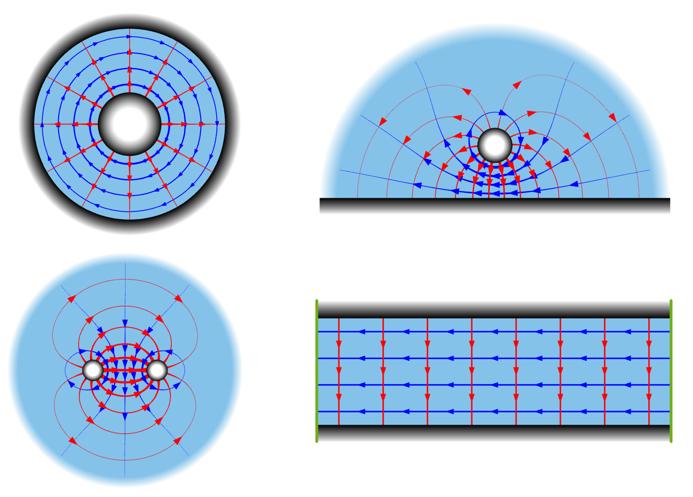 Images of the four true TEM transmission lines. The electric field (red) and magnetic field (blue) are purely in the cross-sectional plane between the two perfect electric conductors (black) and the dielectric within (light blue) is homogeneous. Top left: Coaxial. Top right: Line above plane. Bottom left: Two wire. Bottom right: Parallel plate, with the green lines representing Perfect Magnetic Conductor symmetry conditions.
Once any loss is introduced, either via an Impedance boundary condition or a lossy material, or if there are different dielectrics present, the transmission line becomes quasi-TEM, meaning that there will be some electric, or magnetic, field component in the direction parallel to the line. However, if this component of the fields is relatively small compared to the components in the cross-sectional plane, then even a quasi-TEM line can be modeled using the same excitation types as used for the TEM cases.
The correspondences between true TEM lines and several common quasi-TEM lines are shown in the figures below. Note that other types of lines are possible; they would simply have different shape and/or distributions of dielectric material in the cross section.
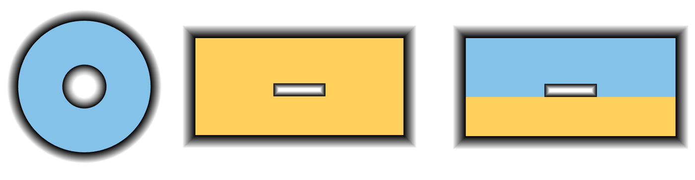 Variations of the coaxial cable line.
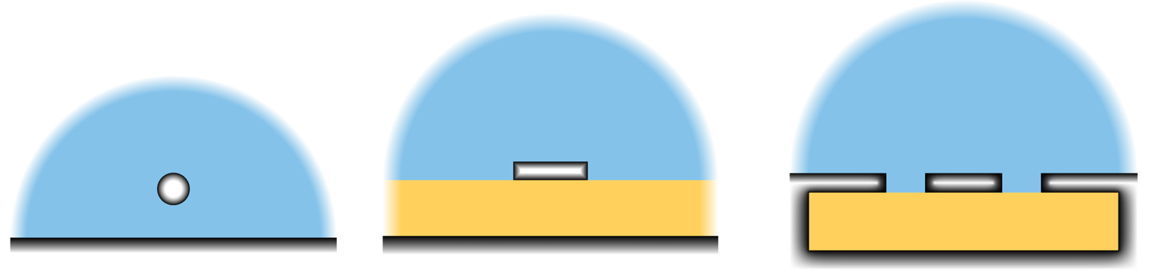 Variations of the line over ground plane.
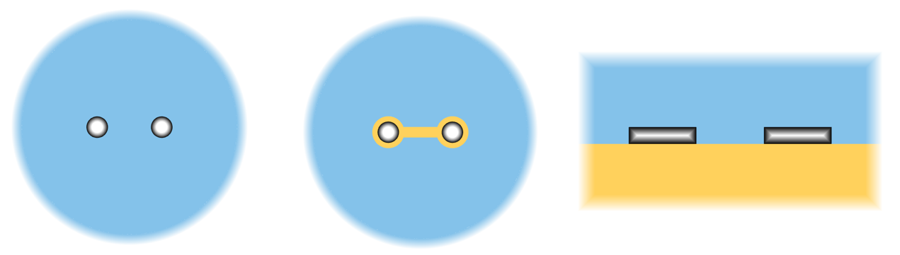 Variations of the parallel wire line.
Many transmission lines are composed of thin metal layers, or traces, patterned on a dielectric substrate. If this metal layer is very thin compared to the trace width, it is often reasonable to neglect the thickness entirely and to simplify the geometry to a surface of zero thickness, as shown in the images below for two common cases.
 Conductors can be modeled as surfaces of zero thickness.
For any type of true TEM transmission line, it is possible to compute the impedance via the Mode Analysis approach shown in the tutorial models Finding the Impedance of a Coaxial Cable and Finding the Impedance of a Parallel Wire Transmission Line. The same approach can be used for quasi-TEM lines. For both TEM and quasi-TEM lines, it is possible to define the voltage as the path integral of the electric field along a line in the cross-sectional plane connecting the two conductors. By convention, one of these conductors is referred to as the ground conductor. For a discussion of voltage and ground, see the corresponding blog post.
In addition, it is also sometimes desired to consider transmission lines operating in common mode or in differential mode. When two conductors are above a ground plane, they can operate in common mode, with both conductors at the same potential, or differential mode, with the conductors at opposite potentials, as represented in the figure below.
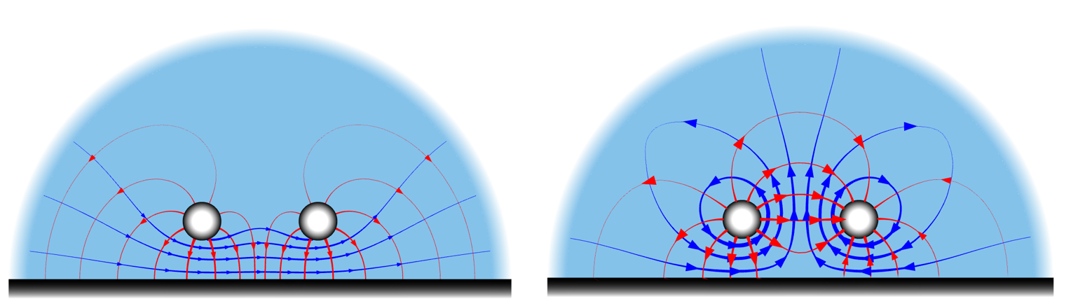 Two conductors above a ground plane in common mode (left) and differential mode (right).
An excited transmission line carries a signal, and this signal will interact with any structure to which the line is connected, leading to some of the incoming signal being reflected back. There can also be losses in the materials, due to radiation, and there can be none, one, or several additional unexcited transmission lines connected to the device through which some fraction of the signal can leave the modeling space. The typical objectives are to compute the S-parameters and to compute the impedance as seen from the excited line of the model. To do so, a set of conditions need to be applied that model the transmission lines within, and external to, the computational domain.
Modeling the Transmission Lines Within the Computational Space
There are four options for modeling the transmission lines within the computational space.
- Perfect Electric Conductor boundaries: Reasonable if the losses in the metal of the line can be neglected. It can be used for both metallic domains with thickness and for modeling traces with zero thickness.
- Impedance boundary condition: Reasonable to use if the skin depth is much smaller than the thinnest dimension of any of the conductors. The volume within the conductors is omitted from the computation.
- Transition boundary condition: For modeling traces where the thickness of the trace is very thin compared to the width, where it is desirable to geometrically model the trace as having zero thickness. It is possible to either specify the thickness, when the skin depth is comparable to the actual thickness of the trace and fields can penetrate through the trace, or enable the Electrically thick layer option, when the skin depth is much smaller than the actual trace thickness, and fields do not penetrate.
- Volumetric model: When the thickness of the conductor is comparable to the skin depth, the volume of the material must be included in the computational space. A boundary layer mesh may be required. If the skin depth is less than ~1/10 of the thickness, consider using the Impedance boundary condition instead.
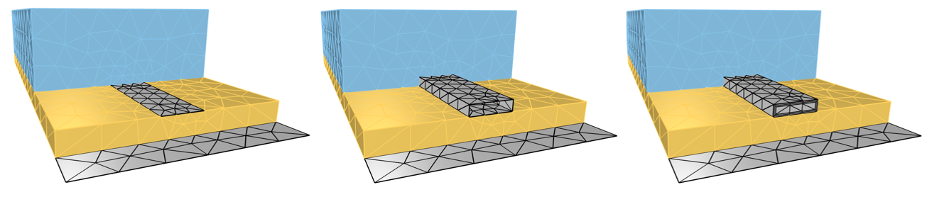 Three side-by-side images showing different types of mesh for a transmission line model.
Left: A thin metal layer of a transmission line modeled via either a PEC or TBC. Center: A thick metal layer modeled via either a PEC or IBC avoids modeling the interior. Right: A volumetric model requires a mesh of the interior of metal, possibly with a boundary layer mesh, depending upon the skin depth.
Three side-by-side images showing different types of mesh for a transmission line model.
Left: A thin metal layer of a transmission line modeled via either a PEC or TBC. Center: A thick metal layer modeled via either a PEC or IBC avoids modeling the interior. Right: A volumetric model requires a mesh of the interior of metal, possibly with a boundary layer mesh, depending upon the skin depth.
Along with the modeling of the conductors, there is the question of how to model the boundaries of the computational domain to surrounding space. If the transmission line is completely enclosed by a metallic shield, such as the coaxial cable, any of the previously described conditions can be used. On the other hand, if the line is unshielded, then there are three options:
- Perfect Magnetic Conductor boundaries: Allows no current to flow along them, and no radiation can leave through them; it can also be thought of as the opposite of the PEC condition. If it is reasonable to assume there is both no shielding and no radiation, this can be used.
- Scattering boundary condition: Type of open boundary condition that approximates a boundary to free space. No currents can flow along these boundaries. Any wave that is propagating approximately normal to an SBC will pass through without reflection, but grazing-incidence waves will be reflected.
- Perfectly Matched Layers: The PML is a type of domain condition that acts as an absorber of any fields that are incident upon them. They are much less sensitive to the angle of incidence (see the blog post "Using Perfectly Matched Layers and Scattering Boundary Conditions for Wave Electromagnetics Problems" but do have specific meshing requirements that increase computational cost, so are only warranted if significant radiation is expected.
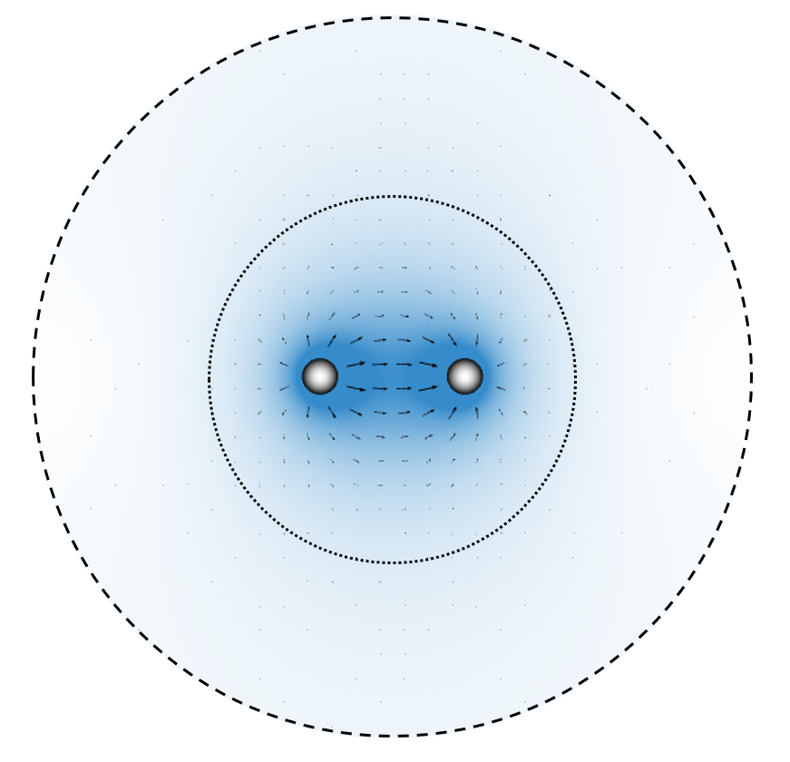
Regardless of which of these options is used, the distance between the transmission line and the boundaries to surrounding space needs to be studied. Although the fields are primarily confined in the space between the conductors, they do extend some distance out to the sides; the so-called fringing effect. The boundaries to free space should be placed where the fringing fields are nearly zero. If these boundaries are placed too close to the line, it can affect the results, as illustrated below. Performing a mode analysis study of such a line is therefore usually a good first step in the overall modeling procedure.
Ports and Lumped Ports for Modeling of Excitations and Terminations
To model the connection to a transmission line outside of the computational domain, there are two classes of boundary conditions that can be used: Ports and Lumped Ports. They can be placed at both interior and exterior boundaries.
Interior boundaries are entirely within the modeling space. The fields are computed on both sides of the boundaries, in contrast to exterior boundaries where the fields exist on only one side. An exterior boundary can also be formed if a region of space is removed from within the modeling domains. These cases are illustrated schematically in the figure below.
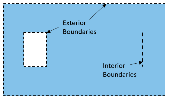
Illustration of exterior and interior boundaries of the modeled domain, in blue.
Overview of the Port Boundary Condition
Port is a generalized boundary condition that can represent both TEM and non-TEM excitations. They can be placed at interior boundaries and can represent either a PEC-backed or a domain-backed one-sided excitation. A PEC-backed excitation means that the signal propagates out of one user-specified side of the boundary, and that any reflected signal will be absorbed by that boundary. Fields impinging upon the other side will be reflected by the PEC boundary. This can be a convenient shortcut to removing a space from within the modeling domain.
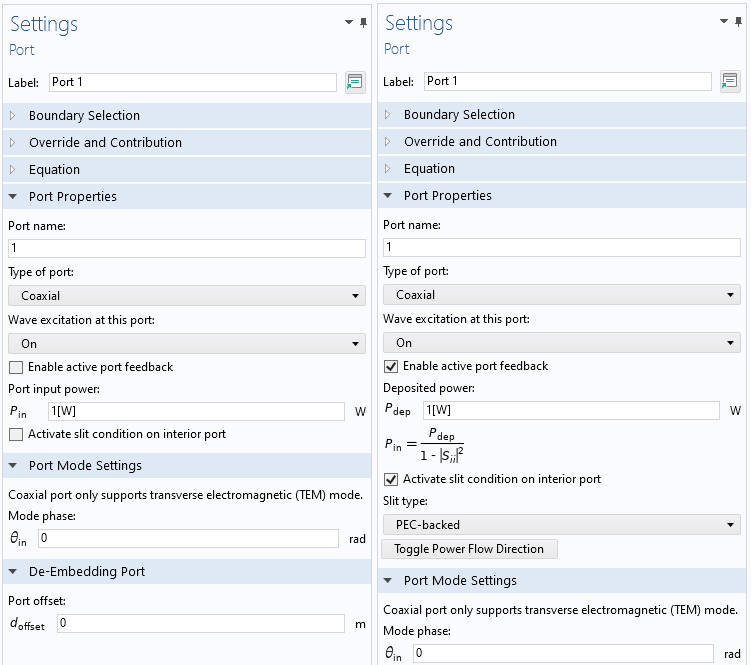
Screenshots of a Port boundary condition.
A domain-backed Port excitation means that the excitation signal will propagate out of one side of the boundary, and any signal reflected back toward the boundary will pass through without reflection and continue propagating through the modeling domain. This option is more commonly used for modeling of waveguides that support multiple TE and TM modes and has lesser application for TEM-type transmission lines.
A Port can inject a signal of fixed power, the default option, which describes a typical microwave power source. There is also the option of enabling active port feedback. The active feedback option is most useful for situations where this is only a single excitation port and it is desired to dissipate a specified amount of power into the lossy material within the modeling domain. It is most commonly used for microwave plasma modeling, but in most other cases, it is reasonable to use a more simplified feedback condition, as described in the blog post "Introducing Goal Seeking into the Segregated Solver".
Finally, the Port boundary condition has a De-Embedding option, which is useful to compute the phase shift due to a nonmodeled length of the transmission line.
Overview of the Lumped Port Boundary Condition
Lumped Ports are meant for modeling of TEM and quasi-TEM lines. They can be placed at exterior or interior boundaries. At interior boundaries, they are two-sided. That is, a signal will propagate out from, and a reflected signal will be absorbed back into, both sides of the lumped port boundaries, which is useful in the context of approximate modeling of terminations.
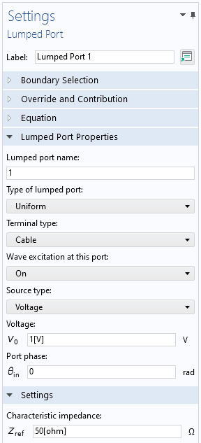
Screenshot of a Lumped Port boundary condition.
A Lumped Port has three types:
- Cable
- Current
- Circuit
The Cable type is for modeling the connection to a transmission line of specified characteristic impedance and can be excited via either a fixed voltage or fixed power. The Current excitation is for exciting via a known current. If this option is used, S-parameters are not available, since there is transmission of signal back into the line. This option is also rarely used in RF applications. The Circuit-type Lumped Port allows connection to an external electric circuit model, as demonstrated in the tutorial model Connecting a 3D Electromagnetic Wave Model to an Electrical Circuit.
Common Settings for Ports and Lumped Ports
Both Ports and Lumped Ports include options for specifying the phase. This option is meant for situations where a model is excited simultaneously from several different transmission lines, and one wants to specify the phase differences between excited lines.
When computing S-parameters, only one Port or Lumped Port can be excited at once. To compute S-parameter matrices, each port needs to be excited individually and the model re-solved. The Frequency Domain Source Sweep Study type automates this process.
When exciting at a single line and sweeping over a wide frequency band, it is often desirable to sample nonuniformly over the bandwidth. The Adaptive Frequency Sweep study type is recommended for such situations, as it will adapt the sampled frequency points based upon the S-parameters.
Modeling Coaxial Cable Terminations
The coaxial cable is most typically modeled using the Coaxial-type Lumped Port. It can also be modeled with the Port condition, although this has no advantages unless there are also higher-order TE or TM modes present. The coaxial lumped port uses the exact analytic expressions of the electric field through the cross section of the cable, and is thus exact if PEC boundaries are used, in the limit of mesh refinement. Practically speaking, having at least two elements in the radial direction is usually sufficient, along with at least eight elements around the circumference.
The coaxial Lumped Port can only be applied to an annular boundary. It can be combined with conductors modeled as PEC, IBC, or as volumes, and should typically only be applied at exterior boundaries.
The Calculator feature within the Coaxial Lumped Port will compute the impedance of the selected annular boundary from the specified dielectric and the inner and outer radius. This should match the specified characteristic impedance, otherwise some reflection will be introduced.
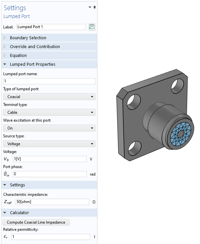
Screenshot of the Coaxial Lumped Port, which must be applied to an annular face (blue) as pictured, along with a representative mesh.
Examples of the usage of this boundary condition include:
- An SMA Connector on a Grounded Coplanar Waveguide
- Connecting a 3D Electromagnetic Wave Model to an Electrical Circuit
- SMA Connectorized Wilkinson Power Divider
- Thermostructural Effects on a Cavity Filter
Modeling of Terminations with Full Geometric Fidelity
To model a general TEM transmission line without geometric approximation, use the Port boundary condition, either of type Transverse Electromagnetic or Numeric with the Analyze as TEM field option enabled. Both cases are shown in the screenshot below. These are typically applied at exterior boundaries, unless higher-order TE and TM modes are also present.
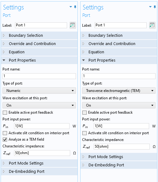
Screenshot of the Port boundary condition. Left: the numeric port option. Right: The TEM option.
Numeric Type Port
The numeric type port is the most accurate way of exciting a transmission line, as it will exactly compute the true propagation constant and fields at a set of cross-sectional faces of the transmission line. It also has the most setup requirements in terms of the geometry.
The Numeric Port with the Analyze as TEM field option will allow two subfeatures to be added that define integration lines for the voltage and current integration paths. The integration line for voltage should bridge the gap between the two metallic domains. The integration line for current should completely encircle one of the metal domains. The numeric port type cannot address the common mode or differential mode cases.
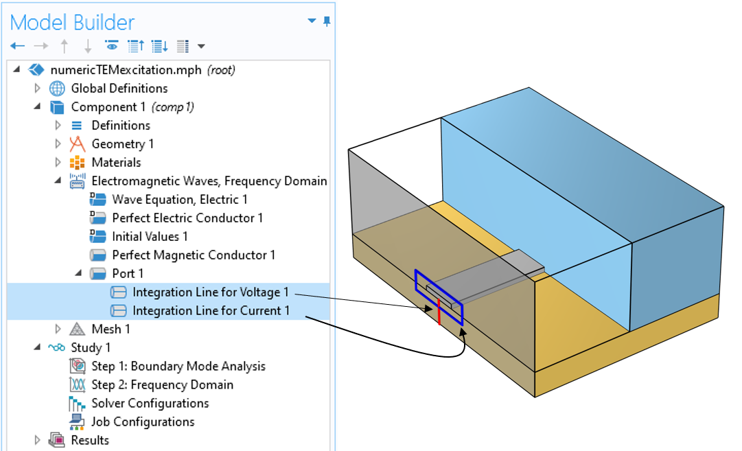 Side-by-side images of the model tree with the integration lines highlighted on the left and an image of the numeric TEM-type port model on the right.
Screenshot of the numeric TEM-type Port boundary condition, with integration lines for voltage and current highlighted. Note also the Boundary Mode Analysis study step.
Side-by-side images of the model tree with the integration lines highlighted on the left and an image of the numeric TEM-type port model on the right.
Screenshot of the numeric TEM-type Port boundary condition, with integration lines for voltage and current highlighted. Note also the Boundary Mode Analysis study step.
When using this boundary condition, it is required that a Boundary Mode Analysis study step needs to be included as the first step within the study. This study step is identical in its settings to the Mode Analysis study performed in a 2D model, such as in Finding the Impedance of a Coaxial Cable.
An example of using this boundary condition is found in the model Notch Filter Using a Split Ring Resonator.
TEM Type Port
When this port type is selected, a Ground and Electric Potential edge condition will appear as subfeatures to the Port feature. Apply the ground condition to all of the edges of one conductor, and the Electric Potential condition to all of the edges of the other conductor. Within the Electric Potential edge condition, there is also the option to specify the potential to be positive or negative, to model lines operating in differential mode. When two physically unconnected edges in the plane are set to positive, this models a line excited in common mode. These edge conditions will be used to solve for the electric fields over the cross-sectional faces of the line. This port type is slightly less accurate that the Numeric port condition, since it does not account for any material losses, but the setup is simpler. It can be combined with any approach for modeling of the line.
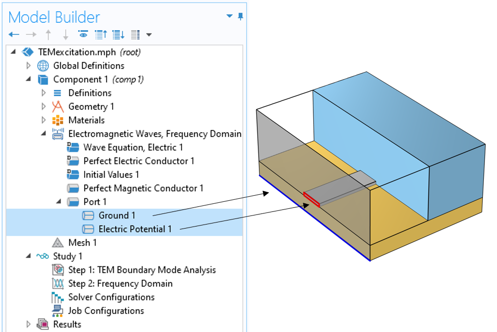 Side-by-side images of the model tree with the Ground Electric Potential subfeatures highlighted on the left and an image of the numeric TEM-type port model on the right.
Screenshot of the TEM-type Port boundary condition, with the Ground Electric Potential subfeatures that are applied to the edges of the metallic regions.
Side-by-side images of the model tree with the Ground Electric Potential subfeatures highlighted on the left and an image of the numeric TEM-type port model on the right.
Screenshot of the TEM-type Port boundary condition, with the Ground Electric Potential subfeatures that are applied to the edges of the metallic regions.
When using this boundary condition, it is required that a TEM Boundary Mode Analysis study step needs to be included as the first step within the study. This will precompute the electric fields on all TEM ports. This study step does require a frequency, which is used to evaluate any frequency-dependent material properties. It does assume that only a TEM mode is present and does no checking for the presence of higher-order modes. It is recommended to check the computed port impedance and ensure that it matches the specified characteristic impedance, otherwise there will be reflections at the port. An example of using this boundary condition is found in the model Modeling of Microstrip Lines with Vias.
Modeling of Terminations with Approximate Geometric Fidelity
There are a number of other options to the Lumped Port that do not introduce as much geometric complexity. Although all of these approaches are approximate, they often provide sufficient accuracy for many modeling purposes.
Uniform
The Uniform Lumped Port is a geometrically simple excitation consisting of a single rectangular surface that must bridge the gap between two sets of conductive surfaces (PEC, IBC, or TBC). This boundary condition imposes a uniform electric field parallel to the direction between the surfaces, comparable to the parallel plate TEM transmission line. It is a quick way of approximating a connection to a physical TEM transmission line, such as a coax, as illustrated in the images below. This boundary condition is applied to interior boundaries, where the fields exist on both sides of the boundary. It is recommended to study the distance between the lumped port boundary and the exterior boundaries of the modeling domain. If the lumped port is placed too close, this can introduce inaccuracy.
Examples of the usage of the uniform lumped port include:
- Coupled Line Bandpass Filter
- Basic Emission and Immunity Analysis of a Circuit Board
- RF Coil
- Microstrip Patch Antenna
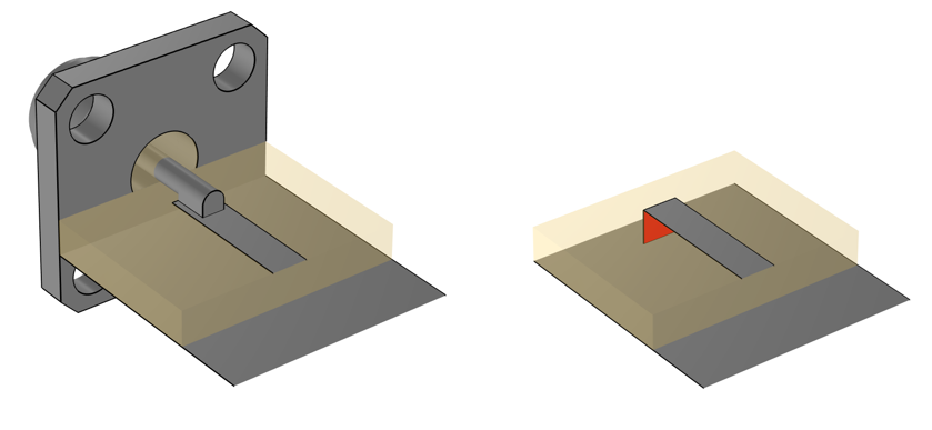
Images showing the correspondence between a coaxial excitation and a uniform lumped port excitation, in red.
Via
The Via Lumped Port must be applied to the boundaries of a set of cylindrical faces that bridge the gap between two sets of conductive surfaces. The interior of the cylinder can be removed from the modeling space, meaning that this boundary is applied on exterior boundaries of the modeling space. The distance between the via lumped port and the other exterior boundaries of the model should be studied to ensure that this does not significantly affect the results.
The via lumped port most typically represents an approximation of the center conductor of a coaxial cable connecting two metal layers. An example of its usage is found in the model Modeling of Microstrip Lines with Vias.
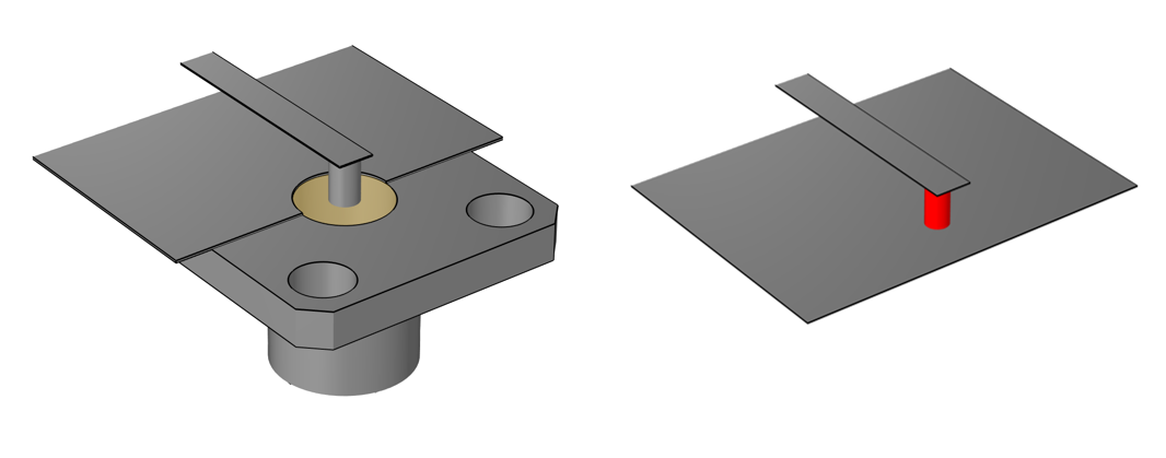 Image showing correspondence between a via lumped port and a coaxial cable.
Multielement Uniform
The Multielement Uniform Lumped Port is most typically used for simplified excitations of coplanar waveguides, as described in the blog posts "Modeling Coplanar Waveguides" and "Simulating an SMA Connector on a Grounded Coplanar Waveguide". This feature is analogous to two Uniform Lumped Ports, where opposite directions of the electric field are specified on the two distinct boundaries. It is applied at interior boundaries, and the distance to the surrounding exterior boundaries should be studied. Examples of its usage include:
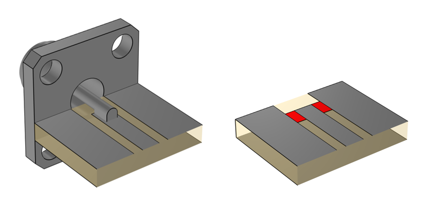
Images showing the correspondence between a coaxial excitation and a multielement uniform lumped port excitation, in red.
User Defined
The User Defined Lumped Port imposes a uniform electric field over a set of surfaces that bridge the gap between two sets of conductive surfaces, and allows to define the direction and dimensions to be entered manually. It is rarely used in practice, as the Uniform and Via types are usually sufficient.
Modeling of a Two-Port Device Within the Model
It is sometimes desirable to model a two-port device within the modeling space. For this, the Two-Port Network feature can be used. This feature can be applied to boundaries representing two Coaxial Lumped Ports or Uniform Lumped Ports. An example of its usage is found in the model Filter Characterized by Imported S-Parameters via a Touchstone File.
Submit feedback about this page or contact support here.