
The Joule-Thomson Effect
What Is the Joule-Thomson Effect?
For several years, James Prescott Joule and William Thomson – both British physicists – worked in collaboration, conducting experiments designed to analyze and advance thermodynamics. In 1852, the researchers made a particularly notable discovery. They found that a temperature change can occur in a gas as a result of a sudden pressure change over a valve. Known as the Joule-Thomson effect (or sometimes the Thomson-Joule effect), this phenomenon has proven to be important in the advancement of refrigeration systems as well as liquefiers, air conditioners, and heat pumps. It is also the effect that is responsible for a tire valve getting cold when you let out the air from a bicycle tire.
The temperature change pertaining to the Joule-Thomson effect can occur when a flowing gas passes through a pressure regulator, which acts as a throttling device, valve, or porous plug. Here, a temperature change is not necessarily desirable. To balance out any Joule-Thomson related temperature changes, a heating or cooling element can be used.
Definitions of Symbols Used to Describe the Joule-Thomson Effect
Before analyzing the Joule-Thomson effect mathematically, you need to be familiar with the nomenclature that is used to describe the effect. The table below provides an overview of the relevant nomenclature:
| Symbol | Quantity | SI Unit |
 |
Specific enthalpy |  |
 |
Heat capacity |  |
 |
Temperature |  |
 |
Pressure |  |
 |
Specific entropy | |
 |
Specific volume |  |
 |
Density |  |
 |
Joule-Thomson coefficient |  |
Understanding the Joule-Thomson Effect
Consider the image below, describing a gas flow that expands through a porous, permeable plug from a higher to a lower pressure state, with thermally insulated walls.
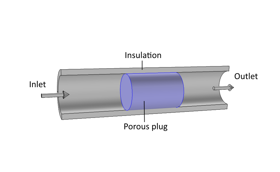 Schematic of throttling through a porous plug.
Schematic of throttling through a porous plug.
Schematic of throttling through a porous plug.
This is an adiabatic throttling process. No heat or mechanical work is exchanged with the environment. Fundamental thermodynamic definitions can be used to develop an energy balance for the flow process into and out of the porous section, with 1 representing the inlet and 2 representing the outlet:

where is the enthalpy and  is the velocity (m/s). Here, any magnetic, electric, and nuclear energy contributions are neglected. For gas flows at moderate velocities, it is safe to disregard the kinetic energy change in comparison to any enthalpy changes:

Therefore, it is evident that the process happens at constant enthalpy – in other words, it is isenthalpic. Most engineers remember from their textbooks that an enthalpy change can be calculated from the material property heat capacity,  , as
, as

At this point, from the equation above, one might jump to the conclusion that if  is 0, then
  must also be 0, assuming that is never 0. Such a conclusion contradicts the experimental findings from Thomson and Joule. The two physicists found that some gases actually change in temperature at throttling. But how can this be explained? The answer lies in some thermodynamic reasoning and the concept of ideal versus real gases. Unfortunately, Eq. (3) is not entirely true; it is a special case for ideal gases (and liquids).
Looking at a more general situation, is a thermodynamic state function. According to the so-called Gibbs' phase rule, the function must have two degrees of freedom for a substance with a fixed composition in one phase. This means that the state of a gas can be exactly determined, provided that the values of exactly two other state functions are known. Determining the enthalpy can be accomplished by determining two other arbitrary state functions. The options include: temperature (), pressure (), entropy (), specific volume (), or internal energy ( ) and more. The only requirement is that two of them are determined.
Here's an example that uses temperature and pressure:

A small change,  , in the enthalpy will, by the chain rule, be:

The indication  represents a partial derivative of with respect to , where is the second degree of freedom selected and is held constant. This can be integrated and replaced with the definition of :

The first term on the right-hand side is the enthalpy change of an ideal gas, and the second term is the additional contribution due to the nonideality of the gas. This can be interpreted as the work that must be exerted to overcome intermolecular forces. An ideal gas, by definition, has no intermolecular forces. For an isenthalpic process, Eq. (4) also helps in the interpretation of any slight temperature change, as it is able to provide the exact amount of thermal energy conversion needed to overcome intermolecular forces.
Revisiting the experiments of Thomson and Joule, the two men found it practical to relate their observations of temperature change at constant enthalpy to something measurable: How much does the temperature change for a small change in pressure, holding the enthalpy fixed? They referred to it as the Joule-Thomson coefficient, :

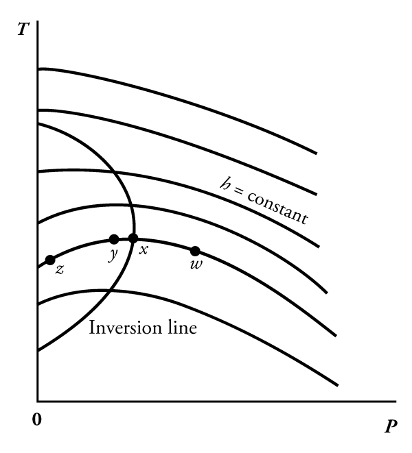
A plot showing the throttling path in a temperature-pressure diagram. The isenthalps are indicated by h = constant. The path of a throttling process goes from a point,  , and moves left along an isenthalp, passing through
  , as well as possibly
  and
and  . Depending on the start pressure and temperature and the final pressure, the temperature can either increase or decrease for a specific gas. The limiting line where a temperature increase changes to a decrease is called the inversion line.
A plot showing the throttling path in a temperature-pressure diagram. The isenthalps are indicated by h = constant. The path of a throttling process goes from a point, , and moves left along an isenthalp, passing through , as well as possibly and . Depending on the start pressure and temperature and the final pressure, the temperature can either increase or decrease for a specific gas. The limiting line where a temperature increase changes to a decrease is called the inversion line.
Thomson and Joule performed extensive work to measure and collect data for common gases. To make Eq. (4) useful in practice, it needs to be related to measurable quantities. The cyclic theorem from mathematics states that

When rearranged, the equation becomes:

Inserting Eq. (6) in Eq. (4) gives the following:

This formula lends itself to evaluation via computer programs or by hand, since the integrated quantities are measurable.
Another useful observation is that a pressure-dependent relation for heat capacity, , can be distilled from the measured data. Reviewing Eq. (6), the  term on the left can be dissected. Combining the first law of thermodynamics with the definition of enthalpy,
  , provides the energy differential:

Taking the derivative with respect to , at constant , on both sides, gives

The well-known Gibbs free energy differential,  , with the so-called Maxwell relations (test for exactness), results in

Inserting Eq. (9) in Eq. (8) produces

Finally, inserting Eq. (10) in Eq. (6) breaks out as

When we have access to a nonideal equation of state,  , it is possible to evaluate this expression using a computational tool.
Summary of the Joule-Thomson Effect and Recommendations
Most gases at normal temperatures are slightly cooled at throttling, with the exception of hydrogen and helium. The internal cooling happens because heat is converted to work that is exerted to overcome intermolecular forces. Ideal gas relations disregard any intermolecular forces and thus miss out on the Joule-Thomson effect. As such, relying only on ideal gas law assumptions when doing flow calculations with computational tools can be risky.
Many engineering textbooks and handbooks include a section on the Joule-Thomson effect as well as tabulated
 data for common gases. This information can be applied to the formula of Eq. (7) and used in both computer simulation programs as well as for calculations by hand.
For more accurate calculations where you need to capture a possible pressure dependency of
, an alternative route is to use a nonideal equation of state, , and evaluate , as in Eq. (11).
Last modified: March 1, 2018
References
- Kenneth Wark, Jr., Advanced Thermodynamics for Engineers (McGraw Hill, Inc., 1995)