Eigenfrequency Analysis
Introduction to Eigenfrequency Analysis
Eigenfrequencies or natural frequencies are certain discrete frequencies at which a system is prone to vibrate. Natural frequencies appear in many types of systems, for example, as standing waves in a musical instrument or in an electrical RLC circuit. Here, we mainly describe the study of eigenfrequencies in mechanical structures, but many of the concepts are generally applicable.
When vibrating at a certain eigenfrequency, a structure deforms into a corresponding shape, the eigenmode. An eigenfrequency analysis can only provide the shape of the mode, not the amplitude of any physical vibration. The true size of the deformation can only be determined if an actual excitation is known together with damping properties.
Determining the eigenfrequencies of a structure is an important part of structural engineering. Some objectives of such an analysis are to:
- Ascertain that a periodic excitation does not cause a resonance that may lead to excessive stresses or noise emission
- Ascertain that a periodic excitation causes a resonance in, for example, a piezoelectric vibrator
- Check if a quasistatic analysis of a structure is appropriate based on the fact that all natural frequencies are high when compared to the frequency content of the loading
- Investigate suitable choices of time steps or frequencies for a subsequent dynamic response analysis
- Provide eigenmodes for a subsequent analysis based on mode superposition
- Provide insight into how design changes can affect a certain eigenfrequency by studying its mode shape
Free vibration at the first natural frequency (440 Hz) of a tuning fork. The displacement is strongly amplified.
Systems with a Single Degree of Freedom
No Damping
As an introduction, we can study a simple system consisting of a mass and a spring, as shown in the figure below.
 Undamped system with a single degree of freedom (DOF).
Undamped system with a single degree of freedom (DOF).
Undamped system with a single degree of freedom (DOF).
The equation of motion for the mass is

If, however, no external force is acting on the mass, nonzero solutions may still exist. It can be immediately verified that

fulfills the homogeneous equation of motion if

Here,  is the natural angular frequency, having the unit rad/s. It is related to the natural frequency
 (unit: Hz) by
  . As long as there is no risk of confusion, a less stringent language is sometimes used, in which is called the natural frequency.
We can interpret the solution above as: Once the process has started, a free vibration can exist at exactly this frequency without any external excitation. If, for example, you stretched the spring and then let go, the mass would vibrate forever at this frequency. In real life, there is always some damping, so ultimately the vibrations would fade away.
The expression for the eigenfrequency above exhibits very general behavior in terms of how stiffness and mass influence eigenfrequencies:

Under a free vibration, the energy in the system is conserved. The kinetic energy of the mass is transformed into strain energy in the spring, and vice versa.
Damped Systems
Assuming that there is also viscous damping in the system, then the equation of motion is

 Single-DOF system with viscous damping.
Single-DOF system with viscous damping.
Single-DOF system with viscous damping.
When analyzing harmonic vibrations, it is convenient to employ a complex notation, where the harmonic functions are represented by  . Such a notation will be used in the following equation. In complex notation, the displacement can be written as
  , where
  is a complex-valued amplitude. In this notation, each time derivative gives a factor
  . The equation of motion can, in the absence of any external forces, then be transformed into

This equation can only be fulfilled for certain values of  (for the nontrivial case
  ), given by

Using the notation
and

the eigenvalue equation can be written as

Here, is called the undamped natural (angular) frequency and  is called the damping ratio.
The eigenvalues, which are the solutions to the quadratic equation above, are

Inserting this value of , the complex-valued displacement is

where  is an arbitrary amplitude.
The periodic part of this expression has the damped natural (angular) frequency  . In front of the harmonic part, there is an exponentially decaying multiplier. Thus, in a damped system, the free vibrations will die out.
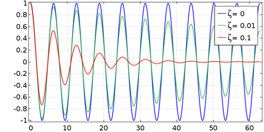 Decaying free vibrations for different damping ratios.
Decaying free vibrations for different damping ratios.
Decaying free vibrations for different damping ratios.
Oscillating solutions can exist only when  . An overdamped system will not resonate at any natural frequency.
Damping processes are, in general, difficult to characterize. The viscous damping used above is popular because of its mathematical simplicity. Another common damping model is hysteretic damping or loss factor damping. This model cannot be explicitly described in terms of time derivatives, but is expressed directly in terms of complex numbers in the frequency domain. The force in the spring is assumed to be out of phase with the displacement, resulting in a complex-valued stiffness. The resulting eigenvalue equation becomes

where  is the loss factor.
The complex eigenfrequency will be
 ,
,
which again is complex-valued. For small values of the loss factor, the exponential factor  gives the decay in amplitude for the oscillations.
Systems with Multiple Degrees of Freedom
A linear system with multiple degrees of freedom (DOFs) can be characterized by a matrix equation of the type

where  is the mass matrix,
  is the damping matrix, and
  is the stiffness matrix. The DOFs are placed in the row vector
  and the forces in
  .
.
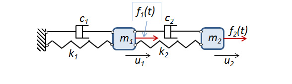 A two-DOF system.
A two-DOF system.
A two-DOF system.
The free vibration problem is then described by the matrix equation

which forms a complex eigenvalue problem. Formally, the eigenvalues can be solved by finding

In practice, other methods are used if there are more than a few DOFs. The number of eigenvalues is usually the same as the number of DOFs. Strictly speaking, the number of eigenvalues equals the rank of the mass matrix.
To each eigenvalue, there is a corresponding mode shape (also known as the eigenmode). When the structure is vibrating at a certain natural frequency, the shape of the deformation is that of the corresponding eigenmode. For the two-DOF system above, the first eigenmode (corresponding to the lowest eigenfrequency) consists of both masses moving in the same direction; whereas in the second eigenmode, the masses move in opposite directions. This is illustrated below for an undamped two-DOF system with  , where the natural frequencies are

and

The corresponding eigenmodes are

and

Here, the maximum element of each eigenmode is arbitrarily chosen to be 1. The two modes are animated below.
The first vibration mode. The relation between the amplitudes of the inner and outer mass is 0.618.
Second vibration mode. The relation between the amplitudes of the inner and outer mass is 1/0.618 and the displacement is in opposite directions.
Note that during the free vibration of an undamped system, all DOFs will reach their respective peak values at the same time. Also, they will pass through the equilibrium position simultaneously. The vibration in the second eigenmode can thus be written as

Orthogonality of Eigenmodes
Two eigenmodes,  and
and  , of an undamped structure can be shown to have the following orthogonality properties:


Since the amplitudes of the eigenmodes are arbitrary, it is possible to choose different types of normalization. A common choice is to use mass matrix scaling, so that

where  is the Kronecker delta.
With this choice of scaling,

where  is the eigenfrequency corresponding to mode i.
If two eigenfrequencies coincide, the corresponding modes are not automatically orthogonal. However, it is always possible to superimpose the eigenmodes so that two orthogonal modes are obtained, and this is almost invariably done in practice.
For damped problems, the eigenmodes will have similar orthogonality properties only for certain forms of the damping matrix . The physical interpretation is that for general damped systems, there will be a cross-coupling between eigenmodes so that energy is transferred between different modes during vibration. The simplest form of the damping matrix that will maintain orthogonality is Rayleigh damping, in which case

where  and
and  are two damping parameters.
Rayleigh damping has no direct physical meaning and is used only because it is mathematically convenient.
Participation Factors
Using modal participation factors is a way to characterize how much a certain mode will be excited by a rigid body acceleration in a certain direction. The participation factor  , with respect to mode i and excitation direction j, is defined as

Here,  is a vector that has the value 1 in all components containing DOFs moving in direction j and 0 in all other components. Note that if mass matrix scaling is used, the denominator has the value 1.
It is also possible to define participation factors for rotational acceleration. In this case, the vector will have a more complicated structure, where the elements depend on the distance from the center of rotation.
Modal Mass
The concept of modal mass sometimes causes confusion. One definition of modal mass is the inner product

When mass matrix scaling is used, this means that the modal mass for each mode is  . Other choices of normalization give other values, so the modal mass in this sense does not really have a physical meaning.
The effective modal mass is a quantity related to the modal participation factor. The effective modal mass for mode i, with respect to excitation in direction j, is defined from the participation factor and the modal mass as

The sum of the effective modal masses in a certain direction j for all eigenmodes equals the total mass of the structure:

The effective modal mass will thus have a physical interpretation. For an acceleration in direction j, it shows how much of the total inertial force can be attributed to mode i. It can be used to estimate how many modes are needed for a good representation in a subsequent response analysis based on mode superposition.
Interpretation of Complex Eigenmodes
As has been noted above, the eigenfrequencies will be complex-valued for damped systems, where the real part contains the angular frequency and the imaginary part provides information about the damping of the mode.
Also, the eigenmodes themselves will be complex-valued. For a damped structure, the eigenmode displacements are no longer in phase at different locations, and the phase information is carried by the complex displacements. If the two-DOF example above is extended by one damper with  , the eigenfrequencies will change to

and

The damping ratio (if small), can be estimated as the ratio between the imaginary and real parts of the eigenfrequency, so it is slightly above 0.2 for both modes. The damped eigenmodes are

and

The difference in phase angles between the two displacement components is 17° for the first mode and 137° for the second. In the undamped case, the corresponding values are 0° and 180°, respectively. The lack of synchronicity is clearly visible in the animation below.
The second eigenmode of the damped system. The displacements of the two masses are no longer in phase.
Continuous Systems
A continuous system — such as a general solid, beam, or plate — will exhibit eigenfrequencies that depend on geometry, material properties, and constraints. A continuous system has an infinite number of eigenfrequencies. For all practical purposes, only a limited number of modes are of interest. Higher modes are unlikely to be excited to a significant extent and often have a higher damping.
For the general case, an eigenmode is a displacement field  defined over the whole body. The orthogonality of the modes can, in the continuous case, be expressed as

where  is the mass density.
Here, the normalization has been chosen with respect to the density (corresponding to mass matrix scaling in the discrete case), but this is not necessary. The mathematical interpretation is that the eigenmodes are orthogonal with respect to an inner product defined with the mass density distribution as a weight function.
Below, the eigenfrequencies for common types of structures are described in more detail.
Beams
For a slender beam with length L, constant bending stiffness EI, and mass per unit length  , the eigenfrequencies can be written as

The coefficient  depends on the support conditions and the number of the mode.
| Support |
|
|---|---|
| Fixed-free (cantilever) |
|
| Pinned-pinned (simply supported) |
|
| Fixed-fixed |
|
| Fixed-pinned |
|


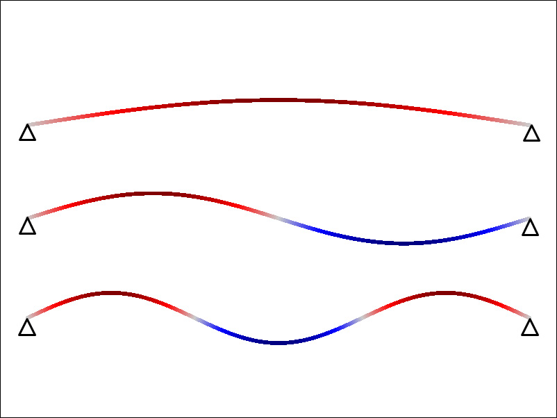 The first three eigenmodes of a simply supported beam.
The first three eigenmodes of a simply supported beam.
The first three eigenmodes of a simply supported beam.
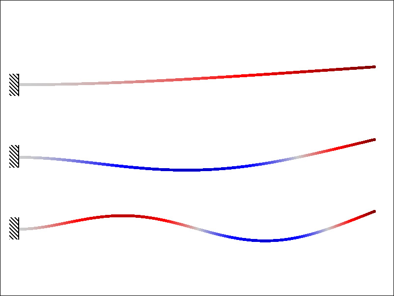 The first three eigenmodes of a cantilever beam.
The first three eigenmodes of a cantilever beam.
The first three eigenmodes of a cantilever beam.
Wires
In a wire, like a guitar string, it is the tensile force that supplies the stiffness. This is why you can tune a guitar by turning the tuning pegs, thus changing the tension in the string. The natural frequencies of a wire are given by the expression

where T is the tensile force, L is the length, and is the mass per unit length.
 A guitar is being tuned.
A guitar is being tuned.
A guitar is being tuned.
Plates
The natural frequencies of plates depend on the bending stiffness of the plate, D, and on the mass per unit area . For an isotropic elastic material, the bending stiffness is

where E is Young's modulus, h is the plate thickness, and  is Poisson's ratio.
The eigenfrequencies and eigenmodes depend on the geometry of the plate and on the support conditions on the edges. The eigenfrequencies are of the form

As an example, the eigenfrequencies of a simply supported rectangular plate with side lengths a and b are

where the indices m and n can be any positive integer value.
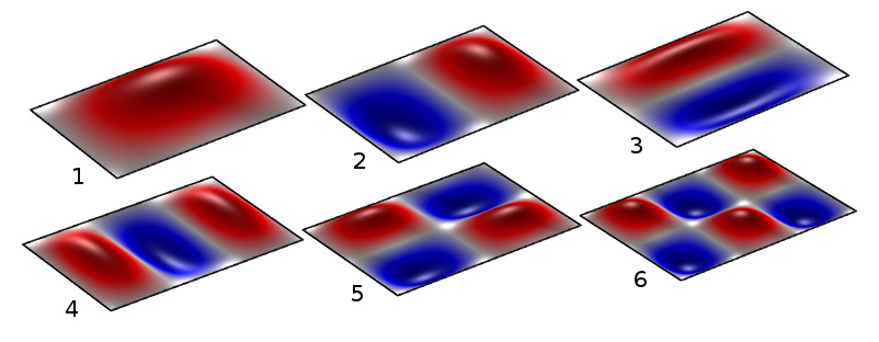 The first six eigenmodes of a simply supported rectangular plate.
The first six eigenmodes of a simply supported rectangular plate.
The first six eigenmodes of a simply supported rectangular plate.
Membranes
Membranes, just like wires, have a stiffness proportional to the in-plane tensile forces. Since the tensile force may not be the same in all directions (and may vary over the membrane), it is difficult to write a general eigenfrequency expression, but the structure is

where T is the in-plane force per unit thickness and is the mass per unit area.
For a circular membrane with radius R and a uniform radial tensile force T, the natural frequencies are

Some of the first values of the coefficients  are given in the table below.
| n = 0 | n = 1 | n = 2 | |
|---|---|---|---|
| m = 1 | 2.405 | 3.832 | 5.136 |
| m = 2 | 5.520 | 7.016 | 8.417 |
| m = 3 | 8.654 | 10.17 | 11.62 |
 The first six eigenmodes of a circular membrane with uniform pretension. The modes correspond to the indices (m,n) = (1,0); (1,1); (1,1); (1,2); (1,2); and (2,0), respectively. Note that modes 2 and 3, as well as modes 4 and 5, are duplicates with identical natural frequencies.
The first six eigenmodes of a circular membrane with uniform pretension. The modes correspond to the indices (m,n) = (1,0); (1,1); (1,1); (1,2); (1,2); and (2,0), respectively. Note that modes 2 and 3, as well as modes 4 and 5, are duplicates with identical natural frequencies.
The first six eigenmodes of a circular membrane with uniform pretension. The modes correspond to the indices (m,n) = (1,0); (1,1); (1,1); (1,2); (1,2); and (2,0), respectively. Note that modes 2 and 3, as well as modes 4 and 5, are duplicates with identical natural frequencies.
Symmetric Structures
Structures that exhibit one or more symmetries will have multiple eigenfrequencies. The corresponding eigenmodes will then not be unique. As an example, consider the second and third mode for the circular membrane previously discussed. These two modes have the same eigenfrequency and the plotted mode shapes are rotated by 90° with respect to each other. However, any orientation of the rotation would also provide a valid eigenmode. In general, it is preferable to select orthogonal mode shapes.
Sometimes, the mode shapes that correspond to multiple eigenvalues obtained from a finite element solution will not have intuitive shapes. Consider a square plate. In a textbook, the modes would probably be displayed as shown below.
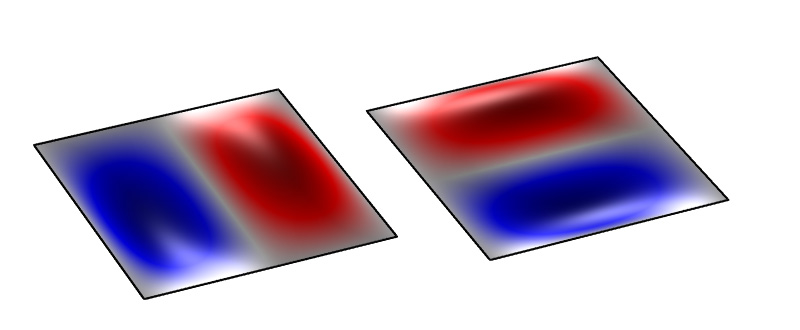 The second and third eigenmodes for a quadratic plate.
The second and third eigenmodes for a quadratic plate.
The second and third eigenmodes for a quadratic plate.
The result from a finite element analysis can, however, be any set of linear combinations of these basic modes. This is exemplified below.
 Another possible choice of second and third eigenmodes for a quadratic plate.
Another possible choice of second and third eigenmodes for a quadratic plate.
Another possible choice of second and third eigenmodes for a quadratic plate.
When analyzing a symmetric structure, it is tempting to make use of the symmetry and model only half or one quarter of the structure. While this is possible, such an approach requires several analyses with different sets of boundary conditions. For example, if one symmetry plane is used, symmetric and antisymmetric boundary conditions must be used.
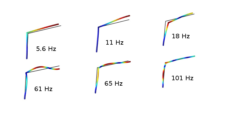
Below, the use of symmetry conditions for a symmetric plane frame is explored. All eigenmodes for the full structure can be retrieved by using two sets of boundary conditions.
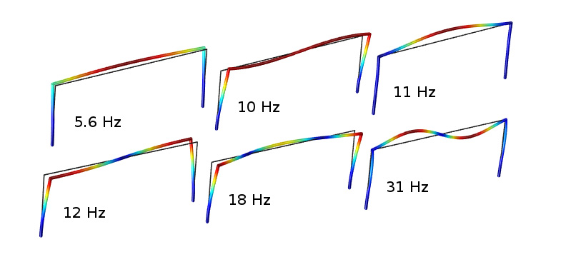 The first six eigenfrequencies and eigenmodes of a soccer goal.
The first six eigenfrequencies and eigenmodes of a soccer goal.
The first six eigenfrequencies and eigenmodes of a soccer goal.
 The first six eigenfrequencies when using half the model and symmetry boundary conditions.
The first six eigenfrequencies when using half the model and symmetry boundary conditions.
The first six eigenfrequencies when using half the model and symmetry boundary conditions.
Structures that have a rotational symmetry will have some eigenmodes that are axially symmetric and some that are not. This means that in general, axially symmetric structures need to be analyzed in full 3D when computing eigenfrequencies.
Modal Stresses
It's not only the displacements of an eigenmode that can be computed and visualized, but also other quantities, like stresses or strains. Just like the displacements, the actual values are arbitrary, but the stress distribution can give insight into how an excitation of a certain mode can affect stresses. This information can be used for design changes when the excitation is known to have a narrow-band frequency content.
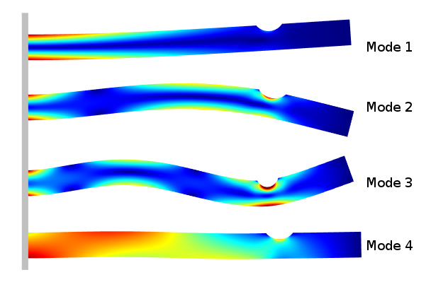 Modal stresses for the first four eigenmodes of a notched cantilever beam. The stress concentration at the notch is mainly activated in the third mode.
Modal stresses for the first four eigenmodes of a notched cantilever beam. The stress concentration at the notch is mainly activated in the third mode.
Modal stresses for the first four eigenmodes of a notched cantilever beam. The stress concentration at the notch is mainly activated in the third mode.
When a structure vibrates, the higher modes usually contribute more to stresses than to displacements. This is because higher modes have more complex shapes and thus larger strains for a certain peak displacement.
Repetitive Structures
Some structures, like fans, can have a large degree of repetitiveness. If we only model a small sector, together with naive cyclic symmetry boundary conditions, we obtain the eigenmodes for a single blade. However, this is not the correct approach, since there is a coupling between the fan blades. It is still possible to perform the analysis on a single sector. The boundary conditions must then be based on Floquet theory. In such a boundary condition, an azimuthal mode number is introduced.
The solution can then be generated for a sequence of azimuthal mode numbers. There is a computational advantage to this approach. Even though we have to perform a number of analyses that match the number of sectors, the computational effort is strictly proportional to the number of sectors. The difference in CPU time between the small one-sector model and the full model is, however, a much larger ratio.
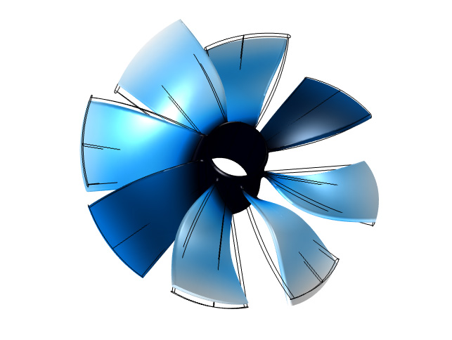 The 14th eigenmode of a fan.
The 14th eigenmode of a fan.
The 14th eigenmode of a fan.
Floquet-type boundary conditions can also be used to compute eigenfrequencies for a large repetitive grid using a model containing only a unit cell.
Unconstrained Structures
A structure does not have to be constrained in order to have natural modes of vibration and corresponding eigenfrequencies. As an example, if you watch a javelin throw in slow motion, you will clearly see how the javelin vibrates in its first bending mode. The unconstrained eigenmodes are sometimes called free-free modes.
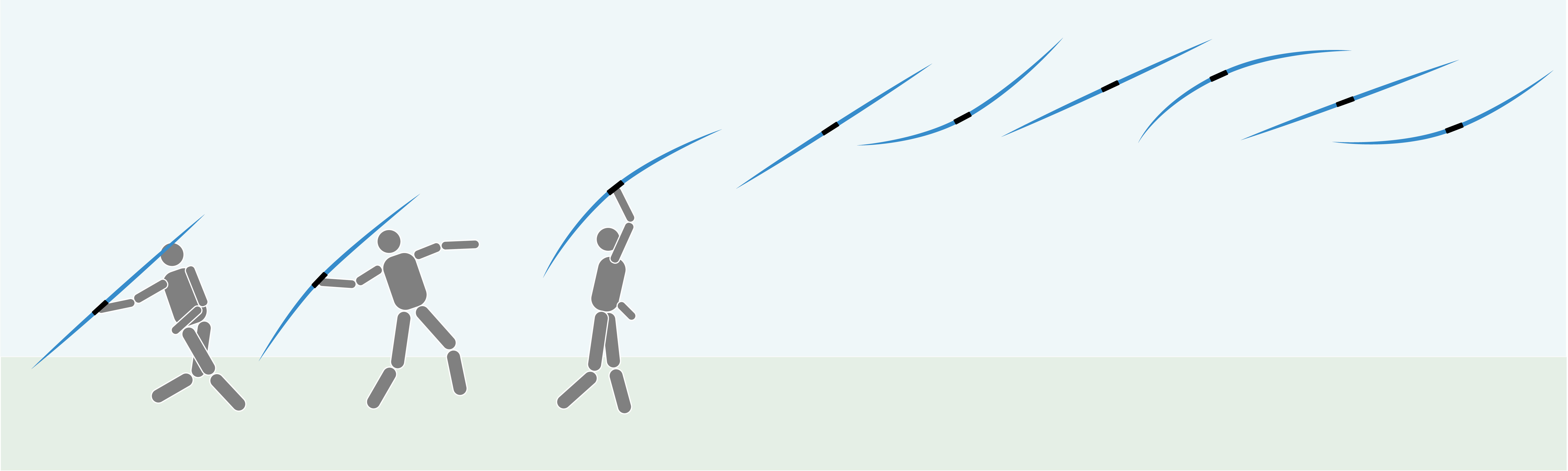 The bending modes of a javelin throw.
The bending modes of a javelin throw.
The bending modes of a javelin throw.
For an unconstrained structure, a number of eigenfrequencies will have the value 0. Zero-valued eigenfrequencies correspond to rigid body motions. For a completely free 3D structure, there will be six rigid body modes. Solving problems like this can be numerically problematic in some formulations.
Stress Stiffening
In general, tensile stresses in a structure will increase its natural frequencies. For membranes and wires, the stress state is actually the sole provider of stiffness. For other cases, like plates, tensile stresses will supply an extra contribution to the bending stiffness. One case where this effect is important is the analysis of fan blades, where the centrifugal forces typically cause a radially directed tensile stress, which increases the natural frequencies.
Similarly, compressive stresses will lower the natural frequencies in a structure.
Published: April 19, 2018Last modified: May 8, 2018