Stress and Equations of Motion
Introduction to Stress and Equations of Motion
When solid bodies are deformed, internal forces get distributed in the material. These are called stresses. Stress has the unit of force per area.
In a bar with a cross section A loaded by an axial force F, the stress in the direction of the force is  . As an everyday observation, we know that thicker objects will be able to sustain a higher force. Thus, stress is an intuitively proper quantity for providing information about how severely loaded a material is.
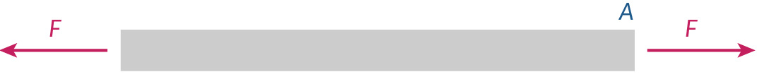 An axially loaded bar.
An axially loaded bar.
An axially loaded bar.
Except for very special cases, as the one shown above, both the magnitude and orientation of stresses vary throughout a loaded body.
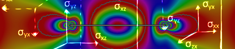
Experimentally determined stress pattern around a rigid inclusion in a soft material. The picture is obtained using photoelasticity. Image by SSMG-ITALY. Licensed under CC BY-SA 3.0, via Wikimedia Commons.
Experimentally determined stress pattern around a rigid inclusion in a soft material. The picture is obtained using photoelasticity. Image by SSMG-ITALY. Licensed under CC BY-SA 3.0, via Wikimedia Commons.
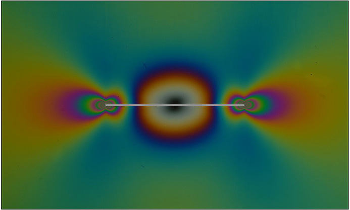
 The corresponding stress pattern, computed using finite element analysis.
The corresponding stress pattern, computed using finite element analysis.
The corresponding stress pattern, computed using finite element analysis.
When the force acts perpendicular to a surface, the stress is called a normal stress. A stress caused by a force acting tangential to a surface is called a shear stress.
Momentum Balance
The internal forces in a body, as given by the stresses, must, together with external forces and inertial forces, be in balance according to Newton's second law.
Let us consider a small surface that consists of the same material particles during the entire deformation process. We assume deformation without loss of continuity in the material, so that no cracks are introduced. Before the deformation, the surface is characterized by the area dA and the normal vector N. After the deformation, these become da and n. The surface is not necessarily a part of the exterior of the body — it can also be a purely conceptual surface anywhere inside the body.
 An infinitesimal surface in the original and deformed configurations.
An infinitesimal surface in the original and deformed configurations.
An infinitesimal surface in the original and deformed configurations.
A surface force acting on the deformed area can be represented as

Here, tn is called traction, while TN is usually referred to as nominal traction, because it relates the force acting in the actual deformed state to the undeformed area.
The traction has the unit force per area. If the area has changed during the deformation, the magnitudes of the two traction vectors are different, but they both have the same orientation.
We can write the nominal traction using its spatial components Ti and the normal vector using its material components NJ. For a discussion about the spatial and material frames, read this page on the analysis of deformation.
Further, we write the traction components as the following linear expansion in terms of the normal vector:

Here and in what follows, summation over repeated indices is assumed. Small and capital indices are used for the spatial and material components, respectively.
Such a representation is sometimes called Cauchy’s law or Cauchy’s formula. This is only possible if PiJ are components of a certain tensor of rank 2.
For an arbitrary undeformed material volume V0, the momentum conservation can be expressed in the following integral form:

where  represents volume forces like gravity or centrifugal forces, and the velocity field is computed from the displacement field,
  , as
, as  .
.
By using Cauchy’s formula and applying the divergence theorem, the surface integral can be converted into a volume integral as:

Since the volume is arbitrary, this gives the following differential form of the momentum balance equation:

Or, using tensor notation:

The tensor P is called the first Piola-Kirchhoff stress tensor. It relates forces acting in the spatial directions to areas in the original undeformed configuration. Thus, its components are given with indices referring to different configurations. Sometimes, such mathematical objects are called two-point tensors. In general, this tensor is not symmetric.
A similar approach can be applied to the traction vector tn and the volume of material in the actual deformed configuration. This will lead to the following representation:

The tensor  is called the Cauchy stress tensor or true stress tensor, as it represents the forces in the actual configuration related to the actual deformed area. This tensor is represented by its spatial components.
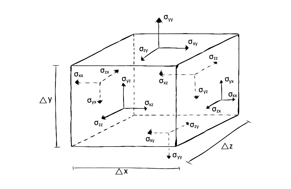
The meaning of the components of the Cauchy stress tensor becomes clear if we consider a small area with the normal vector parallel to one of the spatial coordinate axes; for example, the third one. Then, the normal vector to this area is {0,0,1} and the traction is given by

Thus, the stress tensor component with 33 indices gives the traction vector component in the 3 direction on a plane that has its normal in the same direction. A stress tensor component with two equal indices is called a normal stress or direct stress. The other two stress tensor components provide the part of the traction acting tangential to the plane. Such a component is called a shear stress.
By taking a moment balance for a small cube, it can be shown that the Cauchy stress tensor is symmetric, so that  . This is true as long as there are no volumetric moment contributions. Such materials, which are considered using Cosserat theory, exist. However, they are uncommon.
Since the Cauchy and first Piola-Kirchhoff stress tensors correspond to different representations of the same surface force,

In order to find the relation between the two stress measures, we can use Nanson’s formula for the area change due to deformation. It states that

where F is the deformation gradient tensor and

The volume factor J provides the volume change caused by the deformation. Hence, the stress tensors are connected by

This and similar formulas can be further simplified by introducing a tensor called the Kirchhoff stress tensor, which is defined as  . The Kirchhoff stress tensor has little practical use, but is more of a theoretically convenient quantity.
Mass Conservation and Eulerian Formulation
In terms of the Cauchy stress tensor, the momentum balance equation can be written as

Note that the density in this equation represents the true density of the deformed material. Also, the volumetric force  is the force per deformed volume. The density implicitly depends on the deformation due to the mass conservation as

This added nonlinearity makes this form of the momentum balance equation less interesting from the computational point of view.
By using the velocity and changing the independent variables to spatial coordinates via x = x(X, t), we arrive at

This is the momentum balance in the Eulerian formulation. Such a formulation is typically used in fluid dynamics, where the velocity is treated as a dependent variable.
Mechanical Energy Balance
Multiplying the differential form of the momentum equation by the velocity vector and integrating it over the material gives the following equation:

This equation presents an integral form of the mechanical energy balance. It is also known as the power theorem. The spatial gradient of the velocity is  and the : operator indicates a summation over two indices;
  . The properties of the velocity gradient is discussed in more detail on the Analysis of Deformation page.
The two integrals on the right-hand side of the equation represent the power inputs from the volume and surface forces, respectively. Such power input is the work per unit time done on the material by the respective force.
The terms on the left-hand side are the rate of kinetic energy change and the stress power supplied to the body, respectively. For an elastic material, the stress power is the rate of change of the strain energy density.
By using the relations

the stress power can be represented in the following equivalent form:

Thus, we can say that the first Piola-Kirchhoff stress tensor and the deformation gradient form an energy conjugate pair. Such pairs can also be referred to as power conjugate or work conjugate stress and strain measures.
The velocity gradient can be decomposed into symmetric and antisymmetric parts, called the strain rate tensor (Ld) and spin tensor (Lw), respectively. Since the Cauchy stress tensor is symmetric,  . Hence, the strain measure that is power conjugate to the Cauchy stress is the strain rate tensor. The latter can also be written as

where

is the Green-Lagrange strain tensor. The stress power integral can then be rewritten as:

Here

is called the second Piola-Kirchhoff stress tensor. This is a symmetric tensor that is energy conjugate to the Green-Lagrange strain.
The first and second Piola-Kirchhoff stress tensors are related via:

This formula makes it possible to rewrite the momentum balance equation as:

which together with a constitutive relation of the form

will give a closed system of equations for the displacement vector.
Stress Components on a Rotated Plane
For the axially loaded bar, it is easy to think about the stress  as a scalar number and state that on this bar, only a normal stress exists. The full stress tensor is

This stress tensor has components expressed in a coordinate system with its x-axis aligned with the bar. In any other coordinate system, there will be a mixture of normal stress and shear stress. This can be seen if we consider a conceptual internal surface that is not perpendicular to the axis of the bar. On this surface, there will actually be both normal (σ) and shear (τ) stresses, as indicated in the figure below.
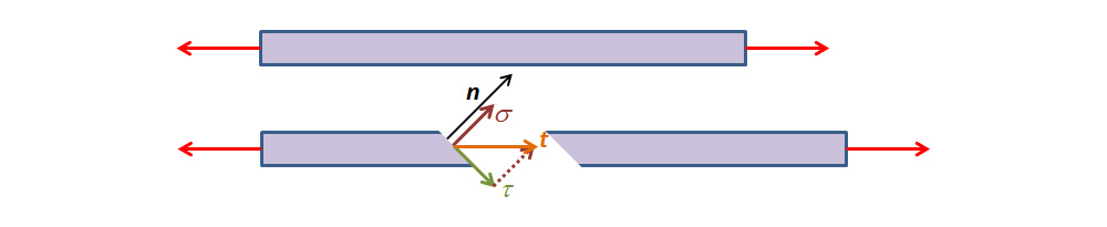 Decomposition of the traction vector into normal and shear stress components.
Decomposition of the traction vector into normal and shear stress components.
Decomposition of the traction vector into normal and shear stress components.
In a rotated system, with its first axis aligned with the normal to the surface, the stress tensor has the structure

where  is the angle between the axis of the bar and the normal to the surface.
A stress state like this is often called uniaxial. However, it is only in a certain coordinate system that it can be represented by a single normal stress component.
Comparing Cauchy and Second Piola-Kirchhoff Stresses
Let us consider an orthotropic material. The material contains fibers in a certain orientation along a straight cantilever beam.
Since it is defined along the material directions, the second Piola-Kirchhoff stress will allow us to visualize the stress in the direction of the fiber, even when the structure is subjected to rotation.
In the figure below, the beam has been bent by a pure moment applied at the tip. We can see the 11-component of both the Cauchy stress and the second Piola-Kirchhoff stress. The bending stress is physically directed along the beam, so the 11-component of the Cauchy stress, which is related to the space-fixed horizontal direction, decreases as the deflection occurs. The second Piola-Kirchhoff stress, on the other hand, has the same through-thickness distribution along the entire beam, also in the deformed configuration.
 The same component of Cauchy stress (above) and second Piola-Kirchhoff stress (below).
The same component of Cauchy stress (above) and second Piola-Kirchhoff stress (below).
The same component of Cauchy stress (above) and second Piola-Kirchhoff stress (below).
The actual value of the second Piola-Kirchhoff stress is more difficult to interpret, since it is not related to either the original or the deformed area.
Published: April 19, 2018Last modified: April 19, 2018