
Convection-Diffusion Equation
Combining Convection and Diffusion Effects
Whenever we consider mass transport of a dissolved species (solute species) or a component in a gas mixture, concentration gradients will cause diffusion. If there is bulk fluid motion, convection will also contribute to the flux of chemical species. Therefore, we are often interested in solving for the combined effect of both convection and diffusion. For a dilute species:
(1)

(2)

Example: Convection and Diffusion in a Microchannel
For a laminar fluid flow at steady state, streamlines that follow the velocity field do not cross each other. The case is not so simple for a turbulent flow, which is discussed in detail below. For the laminar case, since convection transports mass only tangent to the velocity – that is, along streamlines – it cannot lead to mass transfer between adjacent layers of fluid. For a laminar flow at steady state, only diffusion can allow mass transfer normal to the fluid flow.
The distinction between convection tangent to a flow and diffusion normal to a flow can be seen in a simple model of diffusive mixing in a microchannel. In this example, water flows from two inlets at the top left and the bottom left to two outlets at the top right and the bottom right. Because the device is of micrometer scale, the Reynolds number is small and the flow is in the Stokes flow regime. Therefore, the flow profile is symmetric about the vertical as well as the horizontal axis.
Suppose we inlet a concentration of 1 mM (1 mmol/L) of a dissolved chemical species into the bottom-left inlet only; the top-left inlet carries pure water. When the two fluid flows meet at the center line of the channel, there will be a concentration gradient in the vertical (y) direction, and diffusion will carry the solute from the bottom half of the channel to the top half. The operation of the mixer is summarized in the schematic below:
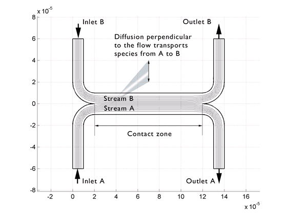 Operation of a microchannel mixer with diffusion normal to the flow.
Operation of a microchannel mixer with diffusion normal to the flow.
Operation of a microchannel mixer with diffusion normal to the flow.
The flow magnitude computed by solving the Navier-Stokes equations is illustrated in the next figure. Note that the streamlines do not cross:
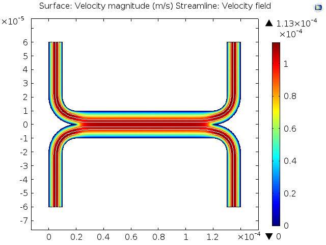 Velocity magnitude (color plot) and streamlines along the velocity field (white lines) in a microchannel. The flow direction is from left to right.
Velocity magnitude (color plot) and streamlines along the velocity field (white lines) in a microchannel. The flow direction is from left to right.
Velocity magnitude (color plot) and streamlines along the velocity field (white lines) in a microchannel. The flow direction is from left to right.
Because of the diffusive mixing, the concentration at the top-right outlet is greater than zero. The concentration at the bottom-right outlet is less than 1 mM. The plot below contrasts the magnitudes and directions of the convective flux (cyan) and diffusive flux (red) at different points along the channel, together with the concentration profile:
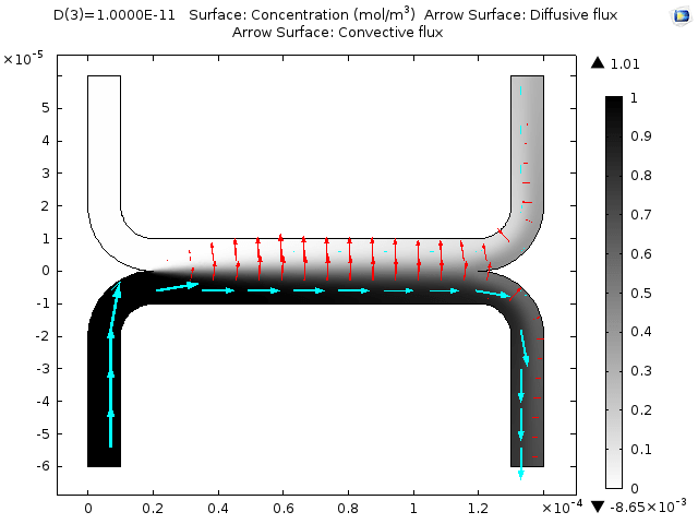 Concentration profile (grayscale), convective flux (cyan arrows), and diffusive flux (red arrows). Convective and diffusive flux magnitudes are indicated by arrow length, on different scales.
Concentration profile (grayscale), convective flux (cyan arrows), and diffusive flux (red arrows). Convective and diffusive flux magnitudes are indicated by arrow length, on different scales.
Concentration profile (grayscale), convective flux (cyan arrows), and diffusive flux (red arrows). Convective and diffusive flux magnitudes are indicated by arrow length, on different scales.
The Péclet Number
It is easy to see in the above example that the degree of mixing can be increased in a number of ways:
A narrower channel, so that the concentration gradients, hence also the diffusive flux, are larger in the vertical direction
A higher diffusion coefficient, so that the diffusive flux is larger
A longer channel or slower flow, so that the fluid takes longer to pass through the channel and there is more time for diffusion
We can work toward quantifying these effects by means of a dimensionless number called the Péclet number (Pe), which is the ratio of the contributions to mass transport by convection to those by diffusion:
(3)

where L is a characteristic length scale, U is the velocity magnitude, and D is a characteristic diffusion coefficient.
The Péclet number for mass transport is comparable to the Reynolds number for momentum transport.
When the Péclet number is greater than one, the effects of convection exceed those of diffusion in determining the overall mass flux. This is normally the case for systems larger than the micrometer scale. However, because the Péclet number is proportional to system size, we find that at small scales, diffusion contributes much more effectively to mass transfer, so mixing can be achieved without stirring. Most forms of mixing (stirring, agitation, static mixers, turbulent flows) act to reduce the length scale over which diffusion must act, hence increasing the local magnitude of mass transfer by diffusion.
Formally speaking, the Péclet number for transport normal to the fluid flow is always zero. This is equivalent to the above statement that diffusion is the only contribution to mass transport between tangent fluid layers. Since the timescale for a flow to traverse a pipe of length L is L/U, the diffusion length, Ldiff , normal to the flow after some distance of flow along the pipe can be found from the diffusion theory
(4)

Considering that there will be a high degree of mixing when the diffusion length scale exceeds the channel width, h, we can state that mixing is effective where:
(5)

That is, a large value of the following dimensionless number:
(6)

The predicted contributions of the variables in a laminar convection-diffusion system agree completely with the simple and intuitive predictions made above for the microchannel.
We can see these same trends in a realistic 3D model of a laminar static mixer, where fixed obstructions are used to bifurcate the flow and hence split the concentration gradient due to the nonuniform concentration at entry. This leads to effective mixing by the half-way point along the channel, as illustrated by the concentration profiles.
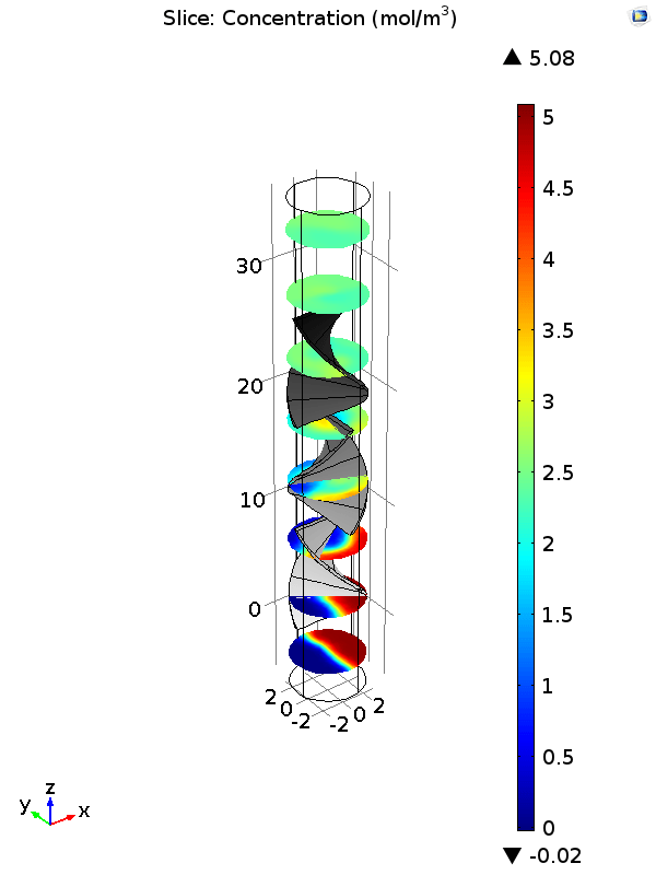 Concentration profiles in slices normal to the flow direction of a laminar static mixer, illustrating the mixing process.
Concentration profiles in slices normal to the flow direction of a laminar static mixer, illustrating the mixing process.
Concentration profiles in slices normal to the flow direction of a laminar static mixer, illustrating the mixing process.
A plot of concentration gradient in a slice along the flow direction (shown below) illustrates how the baffles are positioned to divide and recombine the flow and thereby maximize the volume in which the concentration gradient is large.
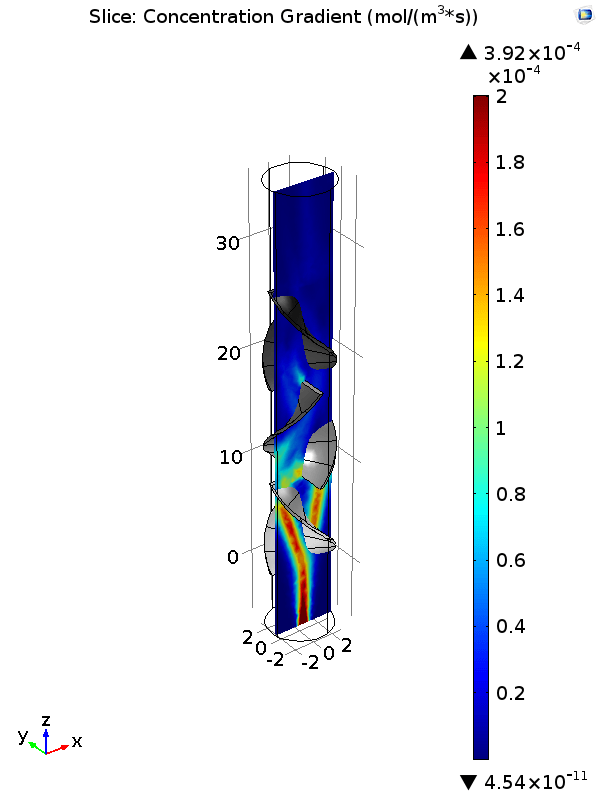 Concentration gradients in a slice along the flow direction of a laminar static mixer, normal to a stepped concentration profile at the inlet.
Concentration gradients in a slice along the flow direction of a laminar static mixer, normal to a stepped concentration profile at the inlet.
Concentration gradients in a slice along the flow direction of a laminar static mixer, normal to a stepped concentration profile at the inlet.
Clearly, the needed diffusion time for mixing between fluid layers is lessened as the diffusion length is shorter. This is why the static mixers, like the one above, are effective at mixing. They increase the surface area of contact between fluid layers with different concentrations of the solute and decrease the length scale of separation between these layers. Although convection may allow the diffusive timescales to be significantly shortened, it is still diffusion that causes the mixing to take place.
Convection-Diffusion in a Turbulent Flow
In a turbulent flow, steady states do not occur. Thus, the simplifications above do not apply. The convective flux acts in the direction of the real, instantaneous velocity of a fluid particle and not the "Reynolds-averaged" velocity, which is often computed for turbulent-flows. Therefore, convection tends to contribute more strongly to mixing in turbulent flows.
It is not practical to use numerical modeling to predict the chaotic and constantly varying instantaneous velocity. Thus, it is normal to express a "convective flux" proportional to the Reynolds-averaged velocity and account for the additional turbulent mixing using an added component of diffusion that is equal to the ratio of the turbulent viscosity, VT, to the turbulent Schmidt number, ScT:
(7)

Here, the Schmidt number is the ratio of observed momentum diffusivity (viscosity) to mass diffusivity. This mathematical approach is analogous to Kays–Crawford model for heat transfer.
Hence, in a turbulent flow, convective mass transport is very important for mixing between noncrossing, time-averaged steady flow streamlines. Again, the consequence of the turbulence is causing the instantaneous streamlines to frequently change position over short length scales, thus increasing the area of contact between different regions of the fluid and allowing diffusion to exchange mass between these regions more efficiently.
Published: January 28, 2015Last modified: March 22, 2018