
Surely you remember the last time you were stuck in bed with the flu. Influenza, commonly known as the flu, can be at the very least an unpleasant experience, but it also claims a lot of casualties every year. Today, public health officials use mathematical modeling techniques to study the flu and other infectious diseases to predict their spread and make informed decisions about public health.
Epidemics: A Dangerous Health Threat
Infectious diseases and epidemics have been a steady issue for humanity over the course of history. The plague pandemics in the Middle Ages, known as the Black Death, killed a third of the population in Europe. The 1918 flu pandemics, immediately after World War I, killed up to 100 million people. Recent epidemic outbreaks of SARS, the flu, and Ebola continue to present a very dangerous threat to our public health. Epidemics also affect the economy and society of both developed and developing countries.
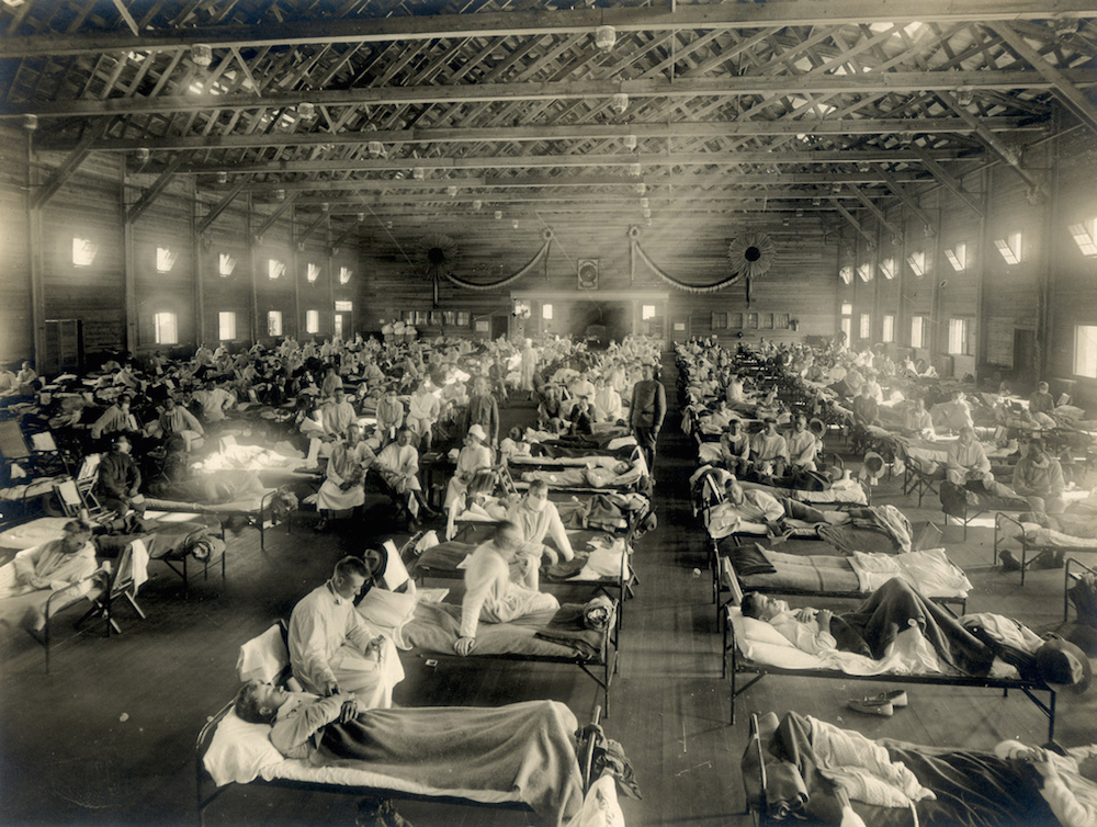
An emergency hospital in Camp Funston, Kansas during an influenza epidemic.
Faced with the threat of disease, medical professionals and public health officials have to make decisions on how to prevent or stop the spread of epidemics, considering questions such as:
- What is the right prevention or control strategy?
- Would mass vaccination help and in what amount of time?
- Should a mass quarantine be imposed on a certain geographical area?
- To halt the spread, should all transportation via planes, trains, and cars be temporarily stopped?
These decisions have to be made quickly and effectively. If not, an epidemic may quickly spread and become a serious threat to global health.
One historical example shows how false control strategies can make the situation much worse. In 1665, there was an outbreak of the bubonic plague in the village of Eyam in England. The story begins with a local tailor who ordered a piece of cloth from London. At that time, London was suffering from an epidemic outbreak known as the Great Plague of London, and the cloth was infested with rat fleas that carry the plague. The plague spread and lasted until the end of 1666, reducing the population of villagers from 350 to 83.
At one point, the villagers turned to a local church leader, who persuaded them to quarantine themselves in their houses. That prevented further spread of the disease in the neighboring villages, but since the villagers remained in close contact with infected rats and stayed among themselves, it caused a second wave of the plague. The disease was transmitted not only between the rats and people, but also from person to person. As a result, the mortality rate in Eyam was much higher than in London. The plague outbreak in Eyam is well documented and there is even a museum that tells the story.
Historical examples can be very informative, but in the end, they can provide only rough guidance. Experiments in epidemiology are also difficult: the data may be incomplete or fully missing, not to mention the serious ethical considerations involved. One solution is mathematical modeling, which is currently used by various national and international public health authorities.
Using the Power of Simulation Against Epidemic Outbreaks
Mathematical models in epidemiology have a storied history that began in the 18th century with another deadly epidemic disease that is now eradicated: smallpox. Smallpox is a severe infectious disease that, at a certain point, had a high mortality rate of over 30%. However, people noted that all who survived had developed immunity against the disease. This led to the invention of a process of inoculation called variolation, which involved deliberately infecting a person with a small amount of the smallpox virus. If everything went well, and the patient had luck, he or she had a high probability of recovery and becoming immune to the disease.
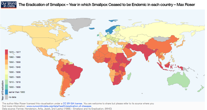
A map showing the eradication year of smallpox in world countries. Image by Max Roser – Own work. Licensed under CC BY-SA 4.0 via Our World in Data. Find more information here.
In 1760, French mathematician Daniel Bernoulli presented his work on modeling smallpox mortality in front of the Royal Academy of Sciences in Paris and showed what effects universal vaccination can have on the spreading of this dangerous disease.
Bernoulli developed one of the first so-called compartmental models of mathematical epidemiology. Others followed and mathematical epidemiology emerged as a discipline, particularly between 1900 and 1935. Notable contributions include that of Sir Ronald Ross, Nobel laureate for the discovery of the mosquito transmission of malaria, and Anderson Gray McKendrick and William Ogilvy Kermack, who developed a compartmental model based on some relatively simple assumptions to predict the behavior of epidemics.
Today, the mathematical modeling of infectious diseases is a dynamic area of research with potentially life-saving impact. Medical researchers and public health physicians use these models to understand the development of an epidemic and answer some fundamental questions, such as:
- How severe will the epidemic be?
- How many people will be affected?
- What is the most efficient control or treatment strategy: quarantine or vaccination?
The models help to identify data gaps and predict the outcome of the epidemic.
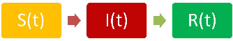
Let’s have a closer look at a variant of the Kermack-McKendrick model, a so-called SIR model. It is a compartmental model that assumes the whole population is divided into different compartments: S for susceptible, the number of people not yet infected by the disease; I for those already infected; and R for removed, those who are either recovered and immune or have passed away. The model considers a rate of flow between different compartments and is formulated through ordinary differential equations. The flow generally looks like this:
In COMSOL Multiphysics, you can type in any algebraic or differential equation and solve it. Let’s use COMSOL Multiphysics to implement the SIR model and calculate one simple example, say, for the flu in winter months.
How to Implement an SIR Model in COMSOL Multiphysics
We use the Global ODEs and DAEs interface, which is available in the core functionality of COMSOL Multiphysics. Let’s assume we have a population of 1000 people in a university or a company where people come in contact with each other often. This population is rather isolated, which means that there are no new people coming in and the main contact happens in that organization. At the beginning of the simulation, there is one infected person with the flu and 999 people who are healthy but susceptible.
We can assume that at the height of the flu season, the infected person infects five other people every day. After they become ill, it takes one to three days until people decide to stay home and rest. Therefore, we can assume that every day, a third of the infected population is removed. We type all of the equations from the SIR model into COMSOL Multiphysics, solve them for a period of 30 days, and analyze the results.
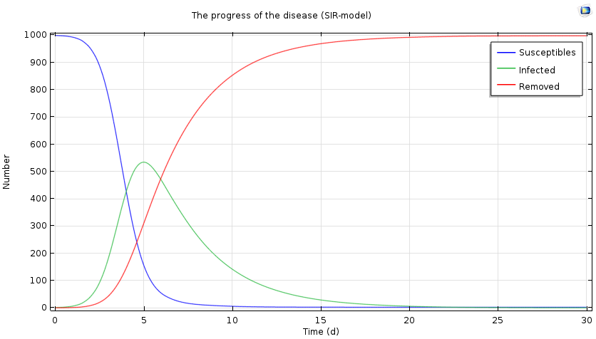
Progress of the epidemic over a period of 30 days, based on the SIR model.
We see a characteristic threshold behavior: If the number of secondary infected persons is sufficiently large, there will be an epidemic and the number of ill people will increase. At the same time, the number of susceptible persons decreases, and ultimately the number of infected persons decreases and approaches zero. In the case above, the epidemic reaches its maximum after five days, with half of the population infected.
This threshold behavior is regulated by the so-called basic reproduction number, a ratio of contact rate and recovery rate that is a fundamental quantity for every disease. However, this number is difficult to determine a priori, since it depends on a lot of factors, such as whether a person is more or less immune to the disease and how people come in contact with each other. This makes the mathematical epidemiology complex, as it is an interdisciplinary field on the crossroads of medicine, computation, statistics, demography, social science, biology, politics, and economics.
Let’s see what happens to the results if every day, 80% of the infected individuals stay home instead of one third. This is what we get:
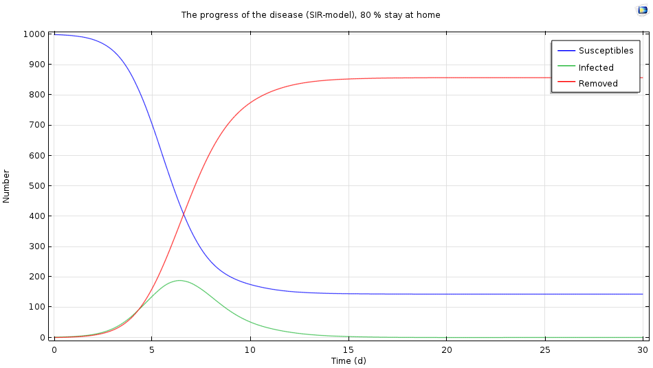
The simulation results when 80% of the infected population stays home after infection.
We see that the epidemic gets a lot milder: There is a maximum level after six days, but fewer than 200 people become infected. In this case, staying at home when infected may be the right strategy.
The SIR model has its limits: it considers a sufficiently large population, not individuals, and the population has to be well mixed. Nevertheless, researchers can already draw some important conclusions. They can derive control mechanisms, which may include the decrease of susceptible people through vaccination or the decrease of contact rate through quarantine.
The SIR model can be applied to viral diseases, such as measles, chicken pox, and influenza. There are also other compartmental models: the SIS model, where all infected people return to the susceptible population (valid for the common cold), or SEIR and SEIS models, which take into account the latent or exposed period. There are also models that describe diseases where the recovery is never fully possible and the patient becomes a carrier; for example, tuberculosis.
These models also have limitations, but can be used to verify either the initial data or hypotheses in a qualitative manner. If we have a look at the figures above and compare them to some real examples, we might notice a discrepancy. Perhaps our population is not so isolated after all, since all employees come in contact with other people outside of their organization, too. There might be some latency period involved, or some people might have already been vaccinated against the flu. There might be transmission vectors involved, such as rats in the case of a plague. Also, the case of the Eyam plague had two waves, meaning that the simple SIR model couldn’t be used.
The reproduction number might also be different. For example, every day, only three or four other people might get infected. A reproduction number, found by comparing model results with real data, can be used to estimate how many people have to be immunized so that disease is no longer endemic. You can find some reproduction numbers here. For example, the model shows that more than 94.4% of people have to be vaccinated against measles to eradicate it. The reproduction number for smallpox is smaller, around 86%, which is why smallpox was chosen for the worldwide eradication campaign.
Using the Heat Transfer Equation for Epidemic Disease Modeling
Liang, Shi, Sritharan, and Wan used a different approach to epidemic modeling in their paper “Simulation of the Spread of Epidemic Disease Using Persistent Surveillance Data“, presented at the COMSOL Conference 2010 in Boston. Using the fact that the spread of epidemic disease can be compared to heat and mass transfer, they used the Heat Transfer Module and the heat transfer equation to formulate a diffusion model to simulate the geographic spread of the disease.
The spread of an epidemic disease is related to a movement of people and interpersonal contacts, much like electron movement and atomic lattice vibrations. They used geographic information such as population, transportation network structure, and the distribution of residences from a sample site in Minneapolis to define medium properties in the heat equation. They also used persistent surveillance data as initial conditions for the transient simulation. In this model, the population density corresponds to the material density; the number of infected and recovered persons corresponds to the heat source and heat loss, respectively; and the contact rate correlates to the thermal conductivity. The researchers also used some boundary conditions available in the Heat Transfer Module for more efficient modeling, such as a thin, highly conductive layer to define local roads, highways, and railroads.
The authors of the paper proposed the introduction of probabilities to achieve the stochastic description of the epidemic spread. From these results, researchers and public health officials can devise public prevention and treatment strategies. There are also other approaches to the modeling delay and other stochastic differential equations, or even more complex models that take into account the movement of every individual, their contacts, and social networks. See, for example, the paper “Networks and the Epidemiology of Infectious Disease“, written by Danon et al.
The Power of Simulation: Same Equations, Different Applications
The fact that the same mathematical and physical models can be applied to entirely different natural or social phenomena is quite astonishing and has encouraged the development of entirely new areas of computational science. The SIR model described above is very similar to the Lotka-Volterra equations, which describe the dynamics between predators and prey. American mathematician Richard Goodwin applied the same model to economics, describing the dynamics of economic cycles and the relationship between wages and unemployment.
The researchers Liang, Shi, Sritharan, and Wan note in their paper that the heat transfer equation and their generic framework can also be applied to forecasting the migration of locust groups and modeling the spread of forest fires. The heat transfer equation can also be applied to financial mathematics and the modeling of stock markets. The scientists have even created other physical models to simulate phase change theory, fluid dynamics, and statistical physics for financial market modeling.
There are even more research applications for this type of simulation work, including opinion dynamics; language development; traffic jams; and even areas such as tax evasion, social segregation modeling, and armed conflicts. Mathematical and physics-based models help to understand and solve other complex issues, not only in technical disciplines, but also in society, especially those difficult or impossible to predict through measurement or observation. In the case of analyzing the spread of diseases, simulation ultimately helps to save lives.
Next Steps
- Learn more about equation-based modeling with COMSOL Multiphysics:
- See 3 examples of equation-based modeling
- Read more about the mathematical modeling of traffic
- Explore the Heat Transfer Module
- See how CFD modeling with COMSOL Multiphysics can help prevent infections
- Read the review paper on the simulation of epidemic diseases in networks: Leon Danon, Ashley P. Ford, Thomas House, et al., “Networks and the Epidemiology of Infectious Disease,” Interdisciplinary Perspectives on Infectious Diseases, vol. 2011, Article ID 284909, 28 pages, 2011. doi:10.1155/2011/284909


Comments (0)