
Ejectors have many applications, such as removing debris in outer space and providing refrigeration at your local supermarket. To improve ejectors for these and other uses, engineers aim to find optimal designs and operating conditions as well as accurately describe the flow within these devices. Simulation can help achieve these goals.
What Is an Ejector?
An ejector is a simple mechanical component with no moving parts that uses momentum and energy transfer from a high-velocity primary jet to induce a secondary flow. During this process, a high-energy fluid (the primary flow) moves through a convergent–divergent nozzle, eventually achieving supersonic conditions.
When the primary fluid leaves the nozzle, it mixes with a secondary flow in an area called a mixing chamber, which is a constant-area duct. This mixing results in a set of complex interactions between the mixing layer and shocks. The fluid expands and decelerates in the mixing chamber and diffuser, a device often placed before the outlet to help recover pressure and return the flow to stagnation. As a result, the fluid speed is reduced to subsonic conditions before it is released into the atmosphere.
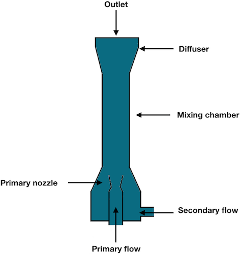
Simple schematic of an ejector.
Ejectors are used for various applications, such as:
- Space debris removal
- Industrial refrigeration (e.g., in supermarkets)
- Gas recirculation
- Thrust augmentation in aircraft propulsion systems
- Vacuum generation
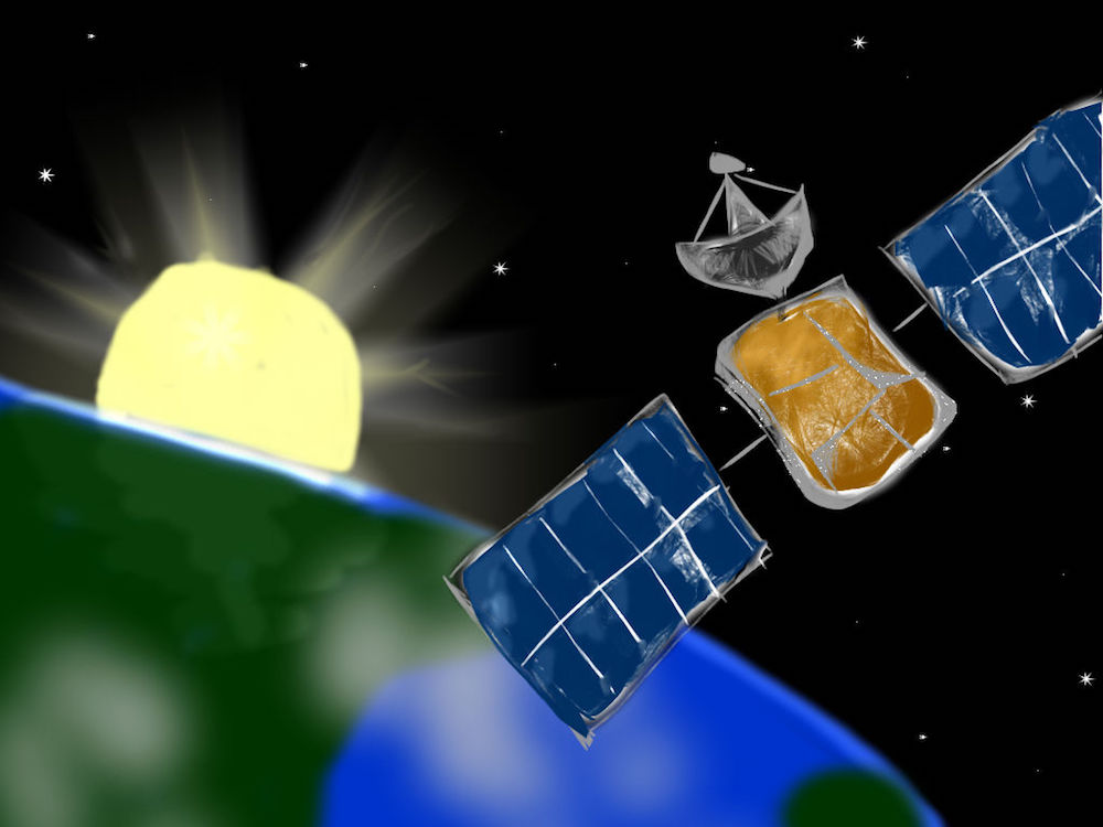
Ejectors can be used to launch nets and capture space debris (like dead satellites) that orbit around Earth and pose a danger to astronauts and space-faring vehicles.
To further advance ejector designs, it’s possible to use simulation to study the compressible turbulent flow within these devices.
Modeling a Supersonic Air-to-Air Ejector with COMSOL Multiphysics®
This benchmark model of a supersonic ejector analyzes air in the primary and secondary streams. For verification purposes, the model definition with geometry, fluid properties, domain settings, and boundary conditions are all taken from scientific literature. Just like in the literature, this example is defined in a 2D axisymmetric coordinate system, since the problem is rotationally symmetric.
For details about the dimensions of this example, check out the model documentation for the supersonic ejector.
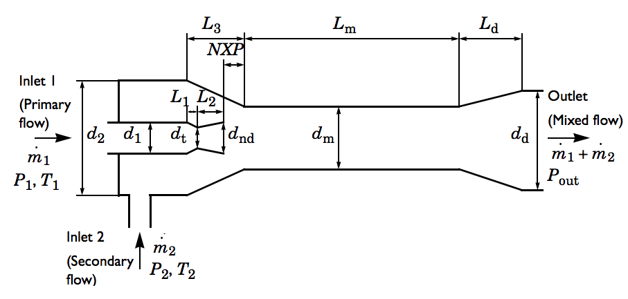
Model geometry of the supersonic air-to-air ejector.
In this example, the pressure of the secondary flow is smaller than the outlet pressure. The secondary flow is induced by the supersonic primary flow exiting the primary nozzle, which can induce a flow with an adverse pressure gradient. This flow is used in vacuum generation, where very low pressures can be achieved in the secondary inlet, and gas recirculation in, for example, fuel cell systems. In the case of recirculation, the COMSOL Multiphysics® software can be used to compute the recirculation mass flows, as seen in the model documentation.
The ejector problem discussed here can be solved using the High Mach Number Flow interface in the CFD Module, which is useful for accurately describing supersonic flows in gases.
Results of the Simulation Analysis
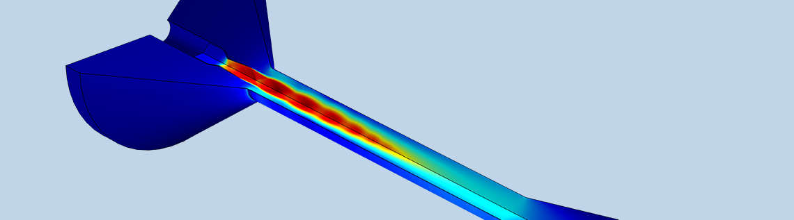
The first result, below, shows that the flow velocity in this example is large enough to cause significant density and temperature variations in the fluid. Further, the flow exceeds a Mach number of 1 in the divergent section of the primary nozzle and in the mixing chamber. The deceleration of the fluid (from supersonic to subsonic flow) occurs through a complex succession of shocks, called a shock train or pseudoshock wave, caused by the boundary layers interacting with the mixing layers. These shocks are clearly seen as shock diamonds in the simulation results.
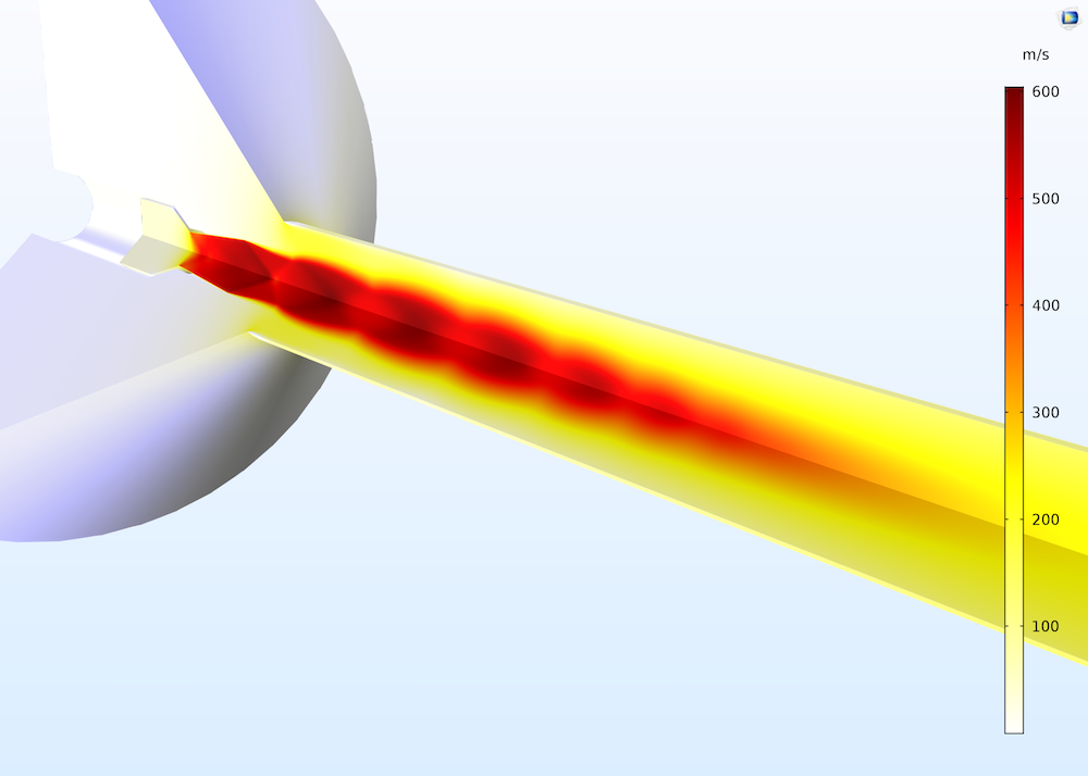
Results showing a typical pattern with shock diamonds in the velocity field. These shock diamonds can also be observed experimentally in the case of reacting flow; for example, when combustion takes place in the flow.
As expected, the primary flow accelerates within the nozzle’s convergent section, achieves sonic conditions in the throat, and expands in the divergent section.


Mach number distribution in the ejector (left) and velocity distribution in the nozzle and mixing chamber (right). Both plots depict shock diamonds.
Meanwhile, the secondary flow behaves like an artificial wall for the primary flow at the outlet of the primary nozzle. This results in virtual nozzle throats and a succession of expansion and compression waves past the mixing zone. Eventually, the flow decelerates within the constant-area duct and returns to stagnation at the diffuser.
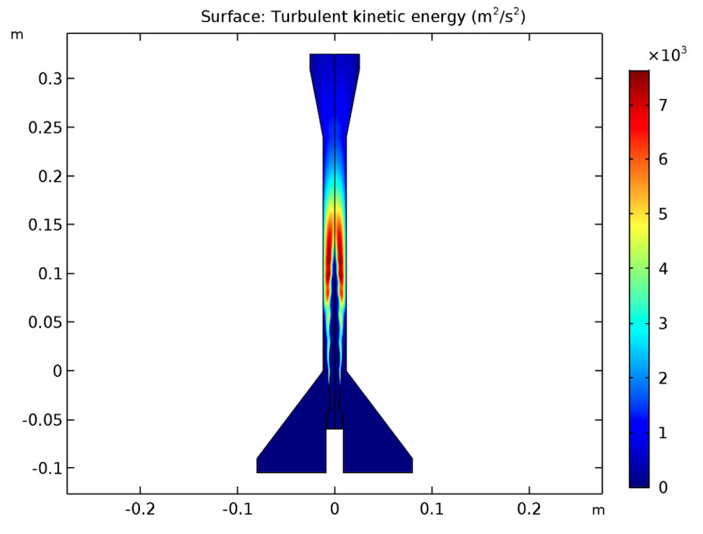
Turbulent kinetic energy distribution in the ejector, showing the two flows combining in the mixing chamber.
Moving on, the plot below analyzes the pressure at the mixing chamber centerline and walls. While it’s true that the multiple shocks cause the flow to switch from supersonic to subsonic at the centerline of the duct, these shocks cannot be detected via wall pressure measurements. The reason the shocks can’t be detected is that the dissipation in the boundary layer can smear out the surface pressures.
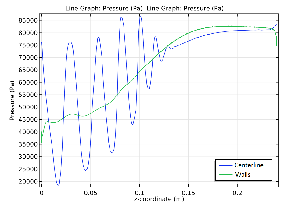
Pressure distribution along the mixing chamber centerline (blue) and walls (green).
Next is the temperature of the ejector. The results here indicate that there are very low temperatures within the ejector. The outlet even has a lower temperature than both of the inlets. This is an important observation for those designing ejectors, especially when they are working with two-phase flows.
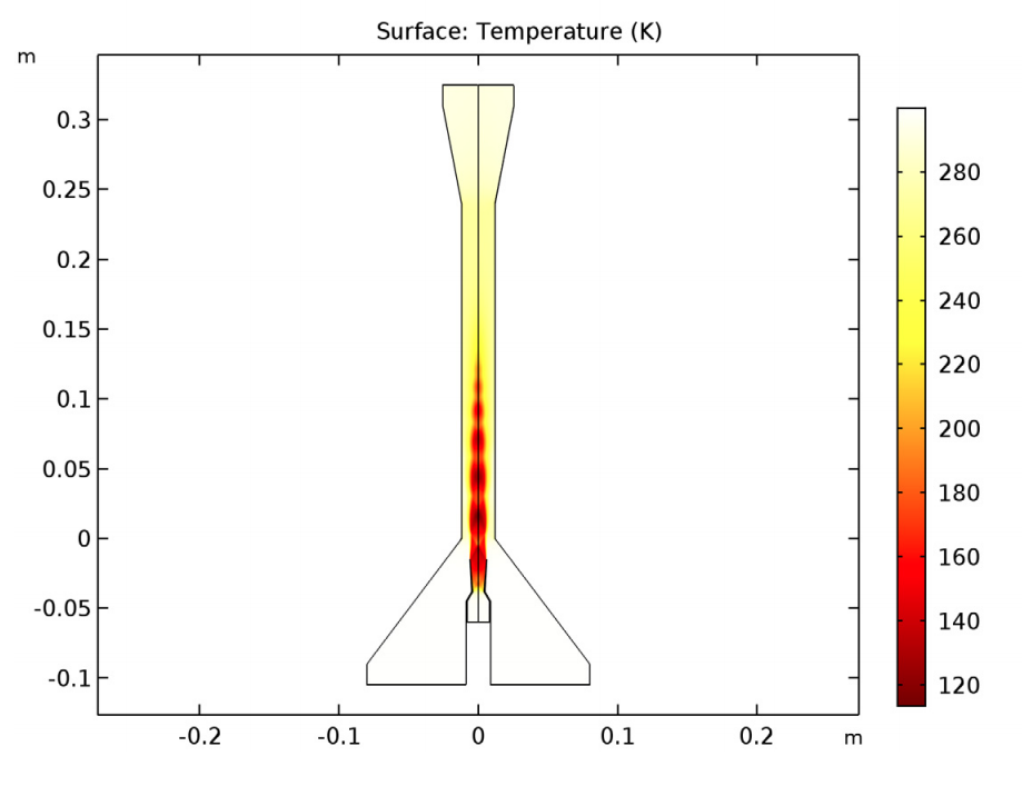
Temperature distribution in the ejector.
The results of the ejector benchmark model correlate well with results found in existing literature, showcasing the ability of the CFD Module to accurately analyze ejectors.
Next Steps
Want to try modeling a supersonic ejector? Get started by clicking the button below. This button takes you to the Application Gallery, where you can use your COMSOL Access account to download the MPH files for the example discussed here.
To learn more about supersonic flows, check out this blog post: How to Model Supersonic Flows in COMSOL Multiphysics®


Comments (0)