
In the past, I’ve received regular requests for the ability to check the view factors used by COMSOL Multiphysics. How accurate are they? What is the impact of a given parameter (mesh size, radiation resolution, etc.) on their accuracy? Good news: Version 5.0 provides new operators for postprocessing that correspond to the operators used to generate surface-to-surface equations. Allow me to demonstrate how to compute geometrical view factors.
About View Factors
Heat transfer computation often needs to include surface-to-surface radiation to reflect reality with accuracy. The numerical tools used to simulate surface-to-surface radiation differ significantly from those used for conduction or convection. Whereas the latter are based on local discretization of partial differential equations (PDEs), surface-to-surface radiation relies on non-local quantities — the view factors between diffuse surfaces that emit and receive radiation.
When surface-to-surface radiation is activated, the heat interface creates a set of operators that are evaluated like the irradiation variables in surface-to-surface radiation. Thanks to these operators, it is possible to retrieve the irradiation variable values and to compute the geometrical view factor in a given geometry.
In this blog post, I’ll explain how to compute geometrical view factors in a simple 3D geometry where analytical values of the view factor are available.
Operators
The new operators in COMSOL Multiphysics version 5.0 offer full access to all of the information used to generate surface-to-surface radiation equations. This is true for even the more advanced configurations, such as radiation on both sides of a shell and multiple spectral bands with different opacity properties.
Let’s start with the simplest case where we assume that surfaces behave like gray surfaces. In this case, we don’t need to distinguish between the spectral bands. We have two operators, one for each face (up or down) of the surfaces. They are as follows:
radopu(expr_up,expr_down)radopd(expr_up,expr_down)
These two operators are designed to be evaluated on a boundary where the surface-to-surface radiation is active. Assuming that the heat interface tag is ht, ht.radopu(ht.Ju,ht.Jd) returns the mutual surface irradiation, ht.Gm_u, that is received at the evaluation point on the upside of the boundary.
Note that ht.Ju and ht.Jd define the radiosity on the up- and downsides of the boundaries, respectively. Similarly, ht.radopd(ht.Ju,ht.Jd) returns the mutual surface irradiation, ht.Gm_d, on the boundary downside.
When multiple spectral bands are considered, a given boundary can be opaque for a spectral band and transparent for another band. Hence, one pair of operators is needed per spectral band. They work exactly like the operator for gray surface and are named as follows:
- The first spectral band:
ht.radopB1u(expr_up,expr_down)andht.radopB1d(expr_up,expr_down) - The second spectral band:
ht.radopB2u(expr_up,expr_down)andht.radopB2d(expr_up,expr_down) - The third spectral band:
ht.radopB3u(expr_up,expr_down)andht.radopB3d(expr_up,expr_down) - etc.
View Factor Definition
Let’s consider two diffuse gray surfaces: S1 and S2. We’ll assume that radiation occurs only on the upside of these surfaces. From a thermal perspective, the view factor between S1 and S2, F_{S1-S2}, is the ratio between the diffuse energy leaving S1 and intercepted by S2 and the total diffuse energy leaving S1.
Using the operators described above, we have
(1)
Note that for clarity, the ht. prefix has been removed.
Assuming that radiosity is the same value on all surfaces, the above definition can be simplified and no longer depends on J. In that case, F_{S1-S2} depends only on the geometrical configuration and no longer on the thermal configuration. Let’s call this a geometrical view factor to distinguish it from the view factor based on thermal radiation.
We now have
(2)
where S1 represents either the surface name or its area and I_{\textrm{S1}} is the function indicator of the surface S1, which returns 1 when it is evaluated on S1 and 0 elsewhere.
Benchmark Case: Two Concentric Spheres
In order to get used to the new operators and check their accuracy, I chose a simple configuration. The geometry consists of two concentric spheres of radius Rint and Rext (with Rint < Rext), as shown below:
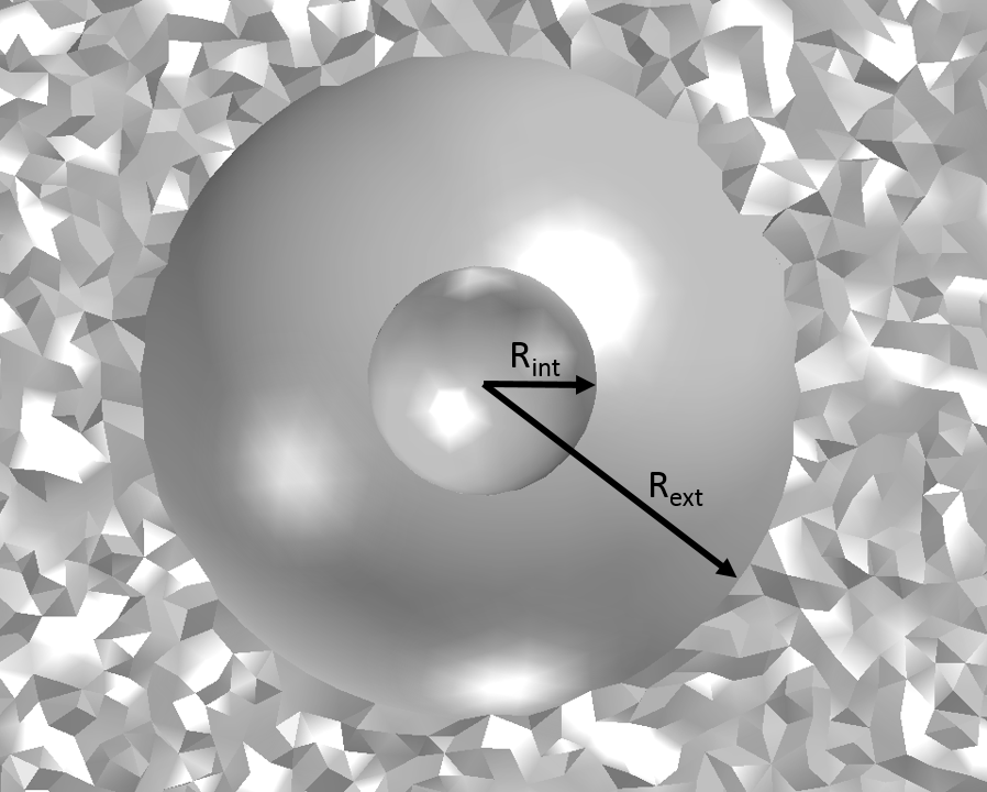
The radiation occurs between the external side of the small sphere and the internal side of the large sphere. The geometrical view factors are:
- F_{S_{\textrm{ext}}-S_{\textrm{ext}}}=1-\left(\frac{R_{\textrm{int}}}{R_{\textrm{ext}}}\right)^2
- F_{S_{\textrm{ext}}-S_{\textrm{int}}}=\left(\frac{R_{\textrm{int}}}{R_{\textrm{ext}}}\right)^2
- F_{S_{\textrm{int}}-S_{\textrm{int}}}=0
- F_{S_{\textrm{int}}-S_{\textrm{ext}}}=1
Here, Sint and Sext represent the interior and exterior sphere, respectively.
Verification in COMSOL Multiphysics
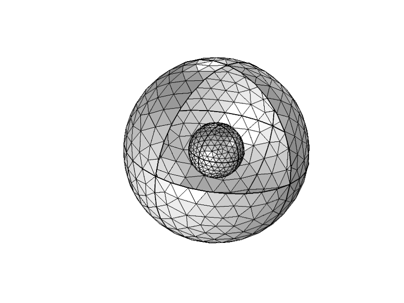
To compute the geometrical view factor in the COMSOL Multiphysics simulation software, we need to add a heat interface with surface-to-surface radiation activated, then draw the geometry and build the mesh.
Then, we don’t really need to run a heat transfer simulation since we are interested in the geometrical view factor. To have access to the radopu and radopd operators is enough to get initial values.
Before doing that, though, we’d better prepare a few tools that will help us with the postprocessing.
Surface Indicator
In the geometrical view factor expression, we have used the surface indicators I_{\textrm{S1}} and I_{\textrm{S2}}. These are defined as Variables in COMSOL Multiphysics and use the Geometric Entity Selection, so that it is 0 everywhere except on the corresponding surface where it is 1. Let’s name them ext and int.
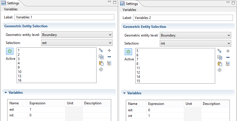
Screenshots of the Geometric Entity Selection settings for the surface indicators.
Integration Over Sint and Sext
Next, we define the integration operators intop_ext and intop_int. They will make it easy to compute surface integrals; for example, the surface of Sext can be evaluated as intop_ext(1).
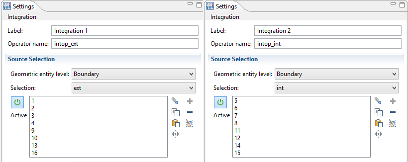
Screenshots of the settings for the integration operators.
Verifying the Radiative Side of Boundaries
We have seen that radiation may occur on the upside, downside, or on both sides of the boundaries. The radiation operators are designed to be able to distinguish the radiation coming from each side. Therefore, we need to check the sides on this model.
We can do this easily via the Diffuse Surface feature, where the radiation direction can be set to “Negative normal direction” (downside) or “Positive normal direction” (upside). Using this option prompts arrows to be automatically displayed to show the direction of radiation leaving the surface. In our example, the radiation occurs on the downside for Sext and the upside for Sint.
Geometrical View Factor Computation
With all these tools available to us, evaluating the view factor using an expression similar to (1) is direct. For example,
(3)
is evaluated in COMSOL Multiphysics syntax with intop_ext(comp1.ht.radopd(0,ext))/intop_ext(1).
Note that the use of radopd is due to the fact that the radiation occurs on the downside of Sext. The first argument of radopd is 0 for the same reason.
(4)
is evaluated with intop_ext(comp1.ht.radopd(int,0))/intop_int(1), where radopd is due to the fact that the radiation occurs on the downside of Sext. But this time, the second argument of radopd is 0 because radiation occurs on the upside of Sint.
I’ve gathered all the results in a table:
| Analytical value | Computed value | Error | |
|---|---|---|---|
| F_{S_{\textrm{int}}-S_{\textrm{int}}} | 0 | 0 | 0 |
| F_{S_{\textrm{int}}-S_{\textrm{ext}}} | 1 | 0.998 | 2e-3 |
| F_{S_{\textrm{ext}}-S_{\textrm{ext}}} | 0.91 | 0.9102 | 2e-4 |
| F_{S_{\textrm{ext}}-S_{\textrm{int}}} | 0.09 | 0.09 | 1e-6 |
Thanks to the radiation operators, we were able to retrieve the geometrical view factor.
Conclusion
With COMSOL Multiphysics 5.0, it is possible to compute geometrical view factors between diffuse surfaces, thanks to dedicated operators. This offers a solution for the requests we received since the surface-to-surface features have been released. But, these operators can do much more. They are flexible enough to provide all terms of the surface-to-surface radiation equation. They may also be used to formulate equations for other quantities.


Comments (10)
Hsin-Liang Chen
October 7, 2016Hi Nicolas,
Thanks for this post. It is quite informative and helpful. But I got a question about how to determine the view factors when the radiosity of the surfaces are not the same. Could you give me a brief idea about how to do this using the “cavity radiation” from the application library as an exmaple? Thanks in advance.
Nicolas Huc
October 19, 2016Dear Hsin-Liang,
What is commonly called “view factor” is determined from the geometry only. So even the radiosity of the surface is not homogeneous the view factor is usually evaluated using equation (2).
If you really want to compute the ratio between the diffuse energy leaving S1 and intercepted by S2 and the total diffuse energy leaving S1 then you have to use equation 1. For the example given here the evaluation of (3) would be intop_ext(comp1.ht.radopd(0,ext*ht.J))/intop_ext(ht.J).
Best regards,
Nicolas
Yi Yan
April 28, 2017Dear Nicolas Huc,
I guess the question Hsin-Liang brought is how your calculation (let’s say equation 2) will be changed if your have two surfaces that are not in the same normal direction. A good example would be a simple right triangular with side lengths 3,4, and 5. I tried to compare the view factors calculated through your method against analytical solution and the match was pretty bad.
Specifically, when I calculate F1-2, it seems like for this integration intop_Surface2(comp1.ht.radopu(1,0)) on surface 2, it will add irradiation from all surfaces(1 and 3) but not just the one (surface 1) I want to calculate. I am not sure how to separate the one I want from all others.
To figure out what’s going on, I would like to ask how the operator radopu( , )/radopd( , ) really work because I cannot find any information on COMSOL Reference Manual.
Also, the two arguments( expr_up,expr_down) in the operator of radopu/radopd, Are they always be 1 or 0? I feel like if the normal directions are not in the same line, then they should be a scale factor based off the angle that two surfaces are forming.
It seems like a very question that is not supposed to ask here but if you have comments or suggestions by any chance, I would greatly appreciate it.
Thanks a lot
Yi
Nicolas Huc
May 31, 2017Dear Yi Yan,
Thanks for your detailed comment! The example you have described is handled with good accuracy. I believe you have highlighted the right thing when you mentioned the two arguments of the radopu operator. It is correct that for view factor computation it is fine to set these arguments 0 or 1. However, the key here is to define a variable, for example I1, that is equal to 1 on the surface 1 and 0 elsewhere. Its definition is similar as for ext and int variables shown on “Screenshots of the Geometric Entity Selection settings for the surface indicators.” figures. With this variable defined, intop_Surface2(comp1.ht.radopu(I1,0)) will return the expected view factors with good accuracy. Feel free to send me your model through the support if needed.
With best regards,
Nicolas
Dheeraj Kumar
December 18, 2017Dear Nicolas
This is an interesting post.
I wanted to know if COMSOL can pre-compute and store view factors if geometry is static? This can significantly speed up (~30 times) parameter estimation or optimization as view factors don’t have to be computed every time. Also, if emissivity is not a parameter being estimated or optimized, effective heat exchange coefficient can also be pre-computed. Of course, large amount of RAM will be required depending on the size of the problem.
Regards
Dheeraj
Nicolas Huc
December 19, 2017Dear Dheeraj,
Thanks for your question.
For any kind of study (time dependent, parametric, etc.) the view factors are computed only once unless the geometry is deformed (due to moving mesh or deformed geometry). In these cases the view factors are reused at every solver iteration.
However if you run the same study multiple times, the view factors is recomputed once per study call. For this reason it is recommended to use the build in parametric sweep rather than using an external script to perform a parametric analysis.
Best regards,
Nicolas
Dheeraj Kumar
December 19, 2017Dear Nicolas
Thanks for the quick response.
I am trying to use one of the optimization algorithms (SNOPT) that comes with the optimization toolbox to estimate some aspects of the model (such as emissivity etc.). View factor calculations appear to be happening in every evaluation even though my geometry doesn’t change. Is there another optimization algorithm or any other way which avoids view factor recalculation every time?
Regards
Dheeraj
Nicolas Huc
December 20, 2017Dear Dheeraj,
When using SNOPT optimization solver the caching of the view factors should be active. However you reported that you have observed a different behavior while solving your model. Could you send this model to me through the support so that we can analyze this model ?
Best regards,
Nicolas
Dheeraj Kumar
December 21, 2017Dear Nicolas
Thanks for the suggestion. I have created the support case: https://www.comsol.com/support/case/2804693/.
Regards
Dheeraj
Francesco Barone
May 9, 2019Dear Nicolas,
I need to calculate the View Factor matrix of a mesh with N triangular surfaces (I have the .stl of that mesh) and export it in a file. This matrix (size N by N) contains the view factor ‘F_ij’ of each triangular surface ‘i’ of the mesh with any other surface ‘j’ of the same mesh.
Is there a way to calculate this matrix with COMSOL? How could I get that? Do I have to use N^2 times radopd or radopu?
Regards,
Francesco