How to Estimate the Parameters of Nonlinear Material Models in COMSOL Multiphysics®

Mechanical systems often contain components that exhibit nonlinear material behavior. Examples include large elastic deformations in seals and gaskets, strain-rate dependence and hysteresis during cyclic loading in rubbers and soft biological tissues, and elastoplastic flow and creep in metals. Together with its Nonlinear Structural Materials Module add-on, the COMSOL Multiphysics® software contains more than one hundred built-in material models that can be used for modeling highly complex material behavior. However, a drawback with these — often phenomenological — models is that they can contain a large number of material parameters, which need to be calibrated for each specific material in order to obtain accurate modeling predictions. In today’s blog post, we will demonstrate how these parameters can be estimated from experimental data obtained from common material tests using nonlinear least-squares minimization techniques.
Common Material Tests
The starting point to estimating material parameters is obtaining relevant experimental data. What should be considered relevant is largely dependent on the type of material and the kind of loads that are expected in the final application, as discussed in a previous blog post. For example, an isotropic linear-elastic material can be characterized with a single uniaxial test. Materials exhibiting strain-rate and loading-history dependence require further experiments, such as relaxation, creep, or cyclic tests at different strain rates. If the component operates at high and/or variable temperatures, the temperature dependence of the material properties might also need to be accounted for.
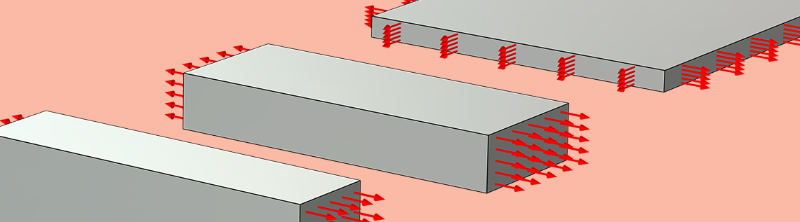
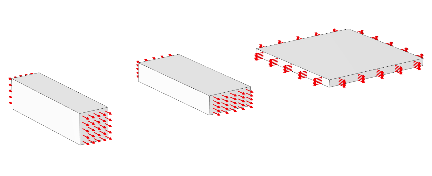
For materials undergoing large deformations, it’s also important to test the material under different states of stress, even if the material behavior is isotropic. Although it can be tempting to calibrate a hyperelastic model to a single uniaxial test, just like for linear elasticity, the prediction of such a model under compressive or biaxial loading might yield unexpected or even unstable material behavior. Instead, a combination of experiments commonly performed for calibrating rubber-like materials involves uniaxial tension, pure shear, and equibiaxial tension tests. Examples of how to realize such experiments for samples of a thin rubber sheet are illustrated below.
From left to right: Uniaxial tension, pure shear, and equibiaxial inflation tests on a thin rubber sheet. The red arrows depict the prescribed displacement and, for the inflation test, the applied inflation pressure.
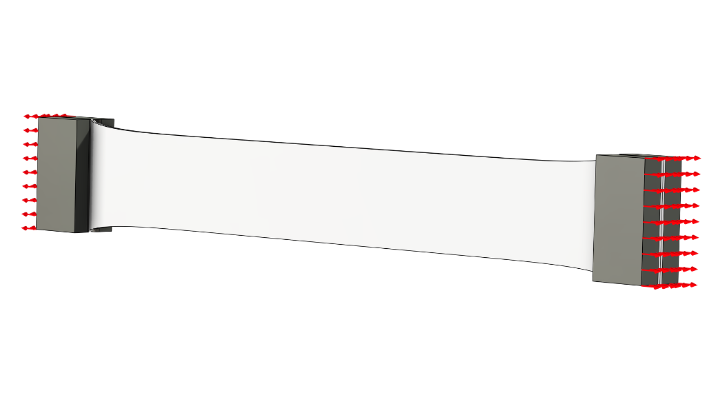
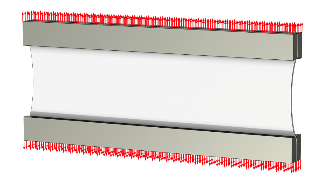
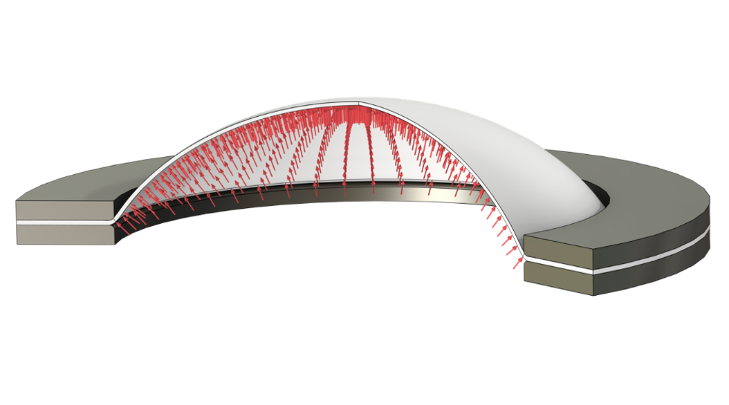
For well-chosen sample aspect ratios, the configurations shown above result in states of homogeneous stress and strain in the center of the samples. These can be estimated from measurable quantities, such as the applied displacements and reaction forces, or the applied pressure and radius of the curvature of the inflated membrane. Material tests that result in homogeneous states of stress and strain are particularly ideal for parameter estimation, since they can be modeled with a single element, which reduces the computational cost significantly.
From left to right: Equivalent homogeneous uniaxial tension, pure shear, and equibiaxial tension load cases.
Nonlinear Least-Squares Parameter Estimation
With experimental data and a choice of material model at hand, we need to select an optimization algorithm that compares the current model prediction with the data and updates the material parameters to minimize the difference. Finding the unknown material parameters, \mathbf{q}^*, thus corresponds to solving a so-called inverse problem. We formulate this mathematically as a weighted least-squares problem,
where \mathbf{W} is a matrix of weights and \mathbf{r} is the so-called defect or residual vector, which contains the difference between the model predictions, \mathbf{y}, and the experimental data, \hat{\mathbf{y}}. The model prediction may depend both explicitly and implicitly on the material parameter, that is, \mathbf{y} = \mathbf{y}(\mathbf{u}(\mathbf{q}), \mathbf{q}), where \mathbf{u} is the solution to the forward problem.
To better illustrate the different components of the least-squares problem, the quadratic form can be expanded to
Herein, N is the number of datasets; Q_n and M_n denote the least-squares error and the number of data points of dataset n, respectively; and P_n(\mathbf{q}; \lambda_m) and \hat{P}_{n,m} denote the model prediction and the experimental data, respectively. The parameter \lambda_m denotes the independent variable for the experiment, such as the time or applied stretch. Furthermore, we have assumed that \mathbf{W} is a diagonal matrix with components 1/s_{n,m}^2, where s_{n,m} are scale factors that weigh the different data points and datasets and ensure that the objective is dimensionless. The least-squares problem may also be augmented by lower and upper bounds on the parameters, which can be used to exclude nonphysical regions of parameter space where the material model is unstable.
In COMSOL Multiphysics®, several optimization algorithms are available for solving least-squares problems. In most cases, the objective is a well-behaved function of the parameters, and the problem can be solved efficiently using the gradient-based Levenberg–Marquardt algorithm. In brief, the Levenberg–Marquardt method updates the parameters iteratively by adaptively alternating between an update step in the gradient descent direction when far from the minimum and a Gauss–Newton step closer to the minimum where near-quadratic convergence can be achieved. An essential quantity in the update algorithm is the Jacobian
which measures the sensitivity of the model prediction to changes in the material parameters. The evaluation of the Jacobian can, in principle, be performed analytically within the optimization solver; however, if the problem is highly nonlinear and the forward model is cheap to evaluate, a finite difference approximation of the Jacobian can often be preferable in terms of robustness and efficiency. When the Jacobian cannot be computed correctly — for example, if the objective is nondifferentiable — the gradient-free bound optimization by quadratic approximation (BOBYQA) algorithm is an alternative that does not require explicit calculation of the derivatives.
Optionally, the Levenberg–Marquardt solver in COMSOL Multiphysics® can also compute confidence intervals as well as the full covariance matrix as measures of the uncertainty in the estimated parameters. This can be particularly useful if you have variance in the experimental data that you want to propagate to the material parameters. For more information, see the Parameter Estimation with Covariance Analysis tutorial.
Nonlinear Material Parameter Estimation Examples
In a previous blog post, we explored how to estimate material parameters for hyperelastic models using analytical expressions of the stress-strain curves derived for two common load cases. However, this approach cannot easily be extended to inelastic material models, for which closed-form analytical solutions often don’t exist. Instead, we can leverage the built-in material models in COMSOL Multiphysics®. Let’s demonstrate this approach for two cases: hyperelasticity and large-strain viscoplasticity.
Parameter Estimation of a Hyperelastic Ogden Model
In the first example, we will calibrate a hyperelastic Ogden model to uniaxial tension, pure shear, and equibiaxial tension data representative of a soft elastomer. The data can be seen below.
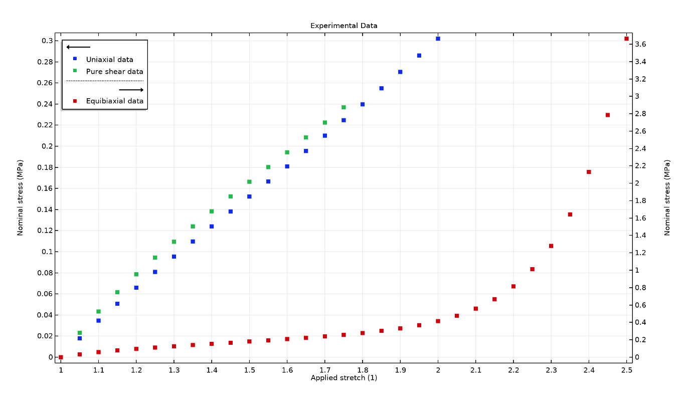
Uniaxial tension, pure shear, and equibiaxial tension data representative of a soft elastomer. Note that the equibiaxial stress is much larger and therefore plotted on a second y-axis.
We assume that the elastomer is incompressible, such that the strain energy density in Ogden’s model reads as
Here, two terms in the strain energy density function are considered, such that the problem consists of solving for the four unknown material parameters \mathbf{q} = (\mu_1, \alpha_1, \mu_2, \alpha_2), as seen in the image below.
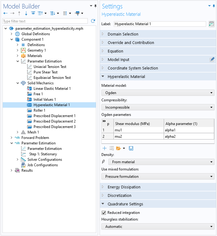
Settings for the incompressible Ogden model with two terms. Note that reduced integration can be used to reduce the computational cost because the load cases are homogeneous.
After setting up the material model, we can import the datasets into results tables and link them to corresponding model expressions using the Global Least-Squares Objective features. The image below shows the settings for the least-squares objective formed from the uniaxial data. The variable comp1.P_ua, used in the Model expression field, is defined as the volume average of the built-in variable for the nominal stress, solid.PxX.
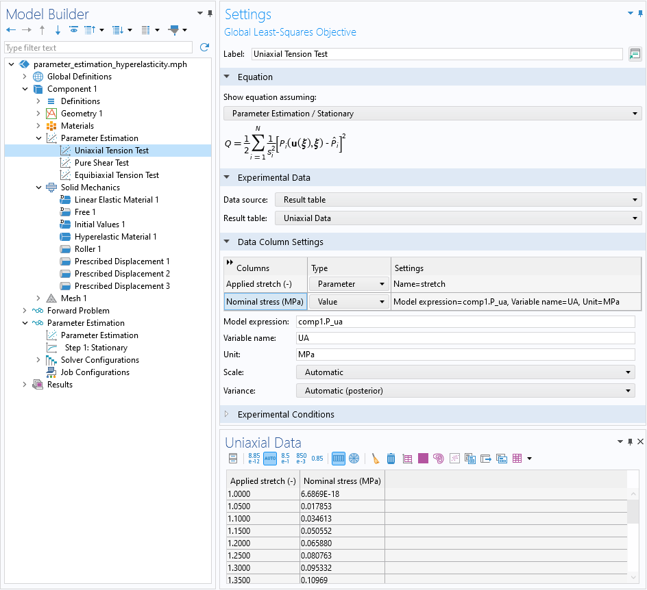
The settings for the Global Least-Squares Objective feature associated with the uniaxial tension data.
In the Parameter Estimation study step, we add the three objectives and specify the material parameters to be estimated. In the Estimated Parameters table, bounds are imposed on mu1 and alpha1 so that they are positive and bounds are imposed on mu2 and alpha2 so that they are negative. These bounds ensure that the material model fulfills the known stability requirements, \mu_p\alpha_p > 0, for Ogden’s model.
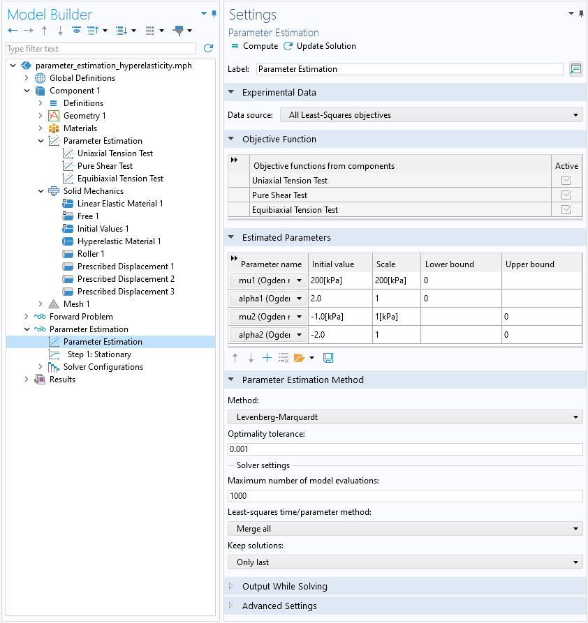
The settings for the Parameter Estimation study step.
The solution progress can be monitored for each iteration of the optimization solver in a plot that compares the current model prediction with the experimental data. As seen in the animation below, the Levenberg–Marquardt algorithm quickly improves the uniaxial and pure shear model prediction and, after a few more iterations, the highly nonlinear equibiaxial response as well.
Parameter Estimation of a Viscoplastic Bergstrom–Boyce Model
In the next example, we consider the more complex Bergstrom–Boyce material model for viscoplastic polymers, which exhibits both strain rate, loading history, and temperature-dependent behavior. Representative stress–strain curves from cyclic uniaxial tension and compression tests at two different strain rates at room temperature are shown below.
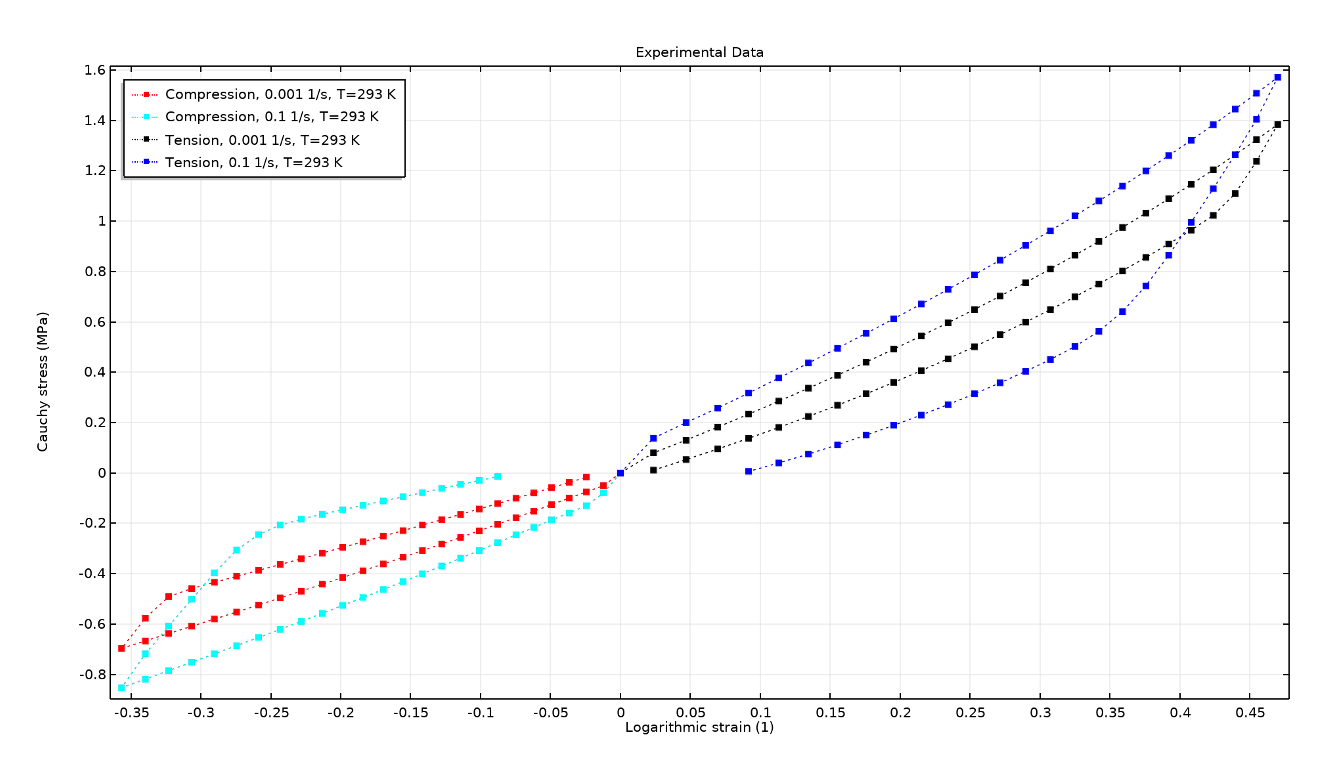
Loading–unloading curves in uniaxial tension and compression at two different strain rates (0.1%/s and 10%/s) for a representative model of a viscoplastic polymer material.
The Bergstrom–Boyce material model is available in COMSOL Multiphysics® version 6.2 in the Polymer Viscoplasticity subnode to a Hyperelastic Material feature. Here, the parent hyperelastic model defines an elastic equilibrium network, while the subnode adds a parallel nonequilibrium network containing both an elastic and inelastic element. In this example, we model the elastic elements with the nearly incompressible Arruda–Boyce strain energy density, and include both strain and stress hardening in the viscoplastic flow. In total, the material model contains six independent material parameters, \mathbf{q} = (\mu_0^\textrm{eq}, N_\textrm{c}, \beta_\textrm{v}, A, c, n): the shear modulus of the equilibrium network, \mu_0^\textrm{eq}; the number of chain segments, N_\textrm{c}; the energy factor between the nonequilibrium and equilibrium network, \beta_\textrm{v}; the viscoplastic flow rate coefficient, A; the strain hardening exponent, c; and the stress hardening exponent, n.
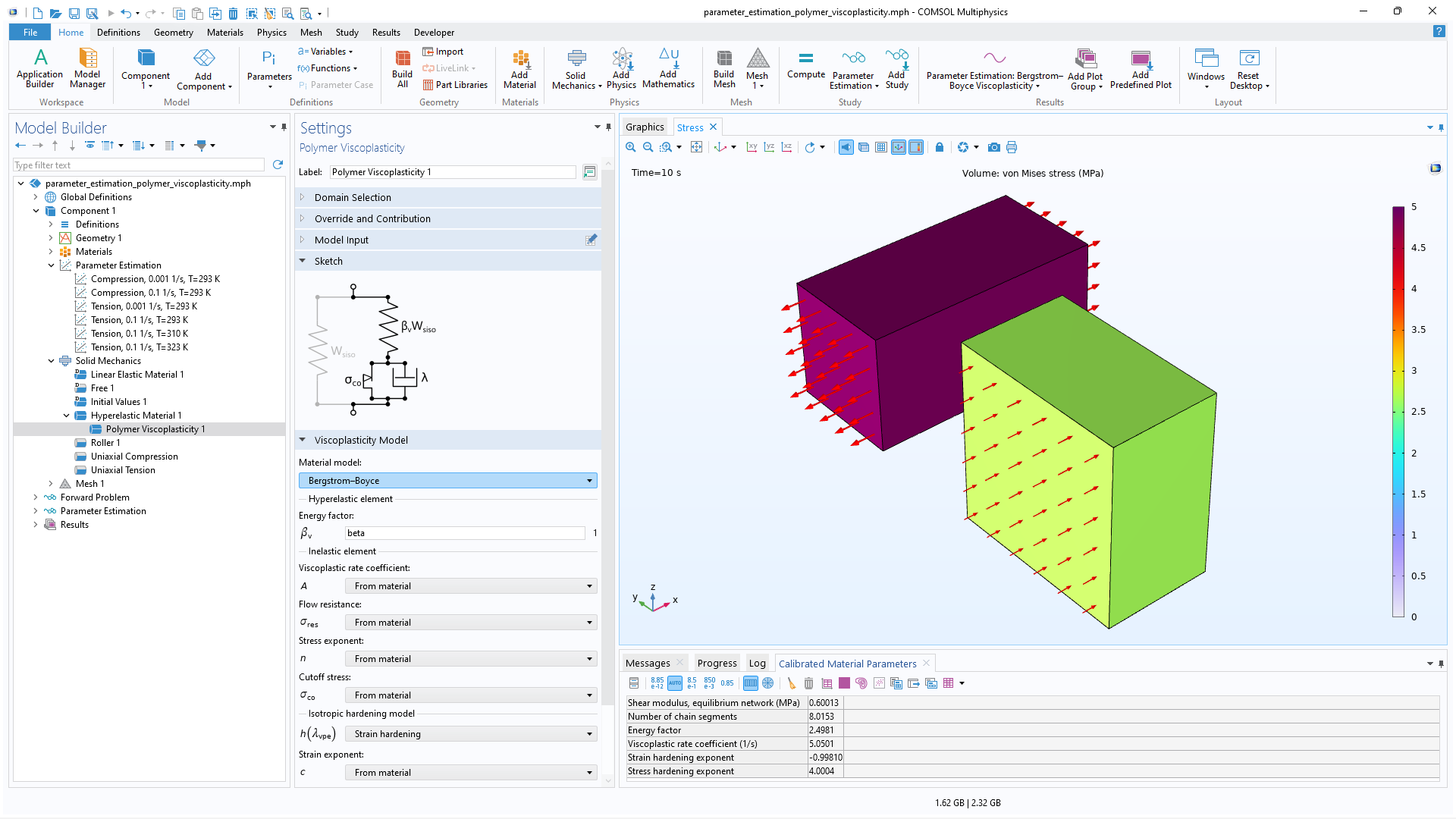
Settings for the Bergstrom–Boyce model in the Polymer Viscoplasticity feature. The Graphics window shows single-element models of the uniaxial compression and tension tests.
The least-squares problem can now be set up and solved in a similar fashion as we did for hyperelasticity. As seen in the animation below, a visually satisfying solution is already obtained after about 5 iterations, even though the optimization solver requires about 12 iterations until convergence. This is because the default termination criteria of the Levenberg–Marquardt solver check if the increment of the parameters or the maximum angle between the defect vector and the Jacobian is smaller than a given optimality tolerance. In the settings of the optimization solver, you can optionally include an additional termination criterion based on the relative change of the defect vector, which can be useful if the solver reaches a relatively flat local minimum in parameter space where improvements in the objective function are small. The default termination criteria are normally more robust than terminating based on defect reduction, though.
Testing the Stability of Your Material Model
After estimating the parameters of a nonlinear material model, it’s good practice to test the material model to ensure that it’s numerically stable. This topic will be covered in detail in Part 2 of this series.
Conclusion and Further Learning
In this blog post, we have demonstrated how to estimate the parameters of nonlinear structural material models in COMSOL Multiphysics® given data from typical material tests. The approach presented is generally applicable to any type of material model and material test data.
To perform parameter estimation of different models yourself, with the help of step-by-step instructions, check out the following models in the Application Gallery:


Comments (0)