
In structural mechanics, there may be situations when you want to implement your own material model. The COMSOL Multiphysics® software gives you the option to program your own material model in C code. The compiled code can then be called from the program using the External Material feature. Here, we demonstrate how to implement an external material model and then use it in an example analysis.
The External Material Functionality
The Nonlinear Structural Materials Module, an add-on product to COMSOL Multiphysics®, provides a plethora of material models, including models for hyperelasticity, isotropic/kinematic hardening plasticity, viscoelasticity, creep, porous plasticity, soils, and more. These material models cover a vast majority of engineering problems within structural analysis.
However, in some situations, the mechanical behavior of a material is not readily expressed in terms of an existing material model. For instance, suppose you developed a specialized material model for a certain alloy and want to use it to solve a large structural mechanics boundary value problem in COMSOL Multiphysics. What do you do?
As a matter of fact, there are three different ways in which you can define your own material:
- Many of the material models have a User Defined option. As an example, you can create your own hyperelastic material by typing in an expression for the strain energy density as a function of the strains directly in the GUI.
- The next level, which is useful when there is no suitable material model that you can tune through a User Defined option, is to express your material model as a set of separate PDEs or ODEs, and enter the appropriate expressions using one of the mathematical interfaces.
- Finally, you can program your own material model in C, using the External Material feature. If the material model is expressed as an algorithm, rather than as a set of equations, this would be the preferred method.
The implementation of a material model as an external DLL can seem like a complex endeavor, but this blog post demonstrates how to implement an elastoplastic material model in COMSOL Multiphysics using hands-on steps that you can follow.
Implementing an Elastoplastic Material Model in COMSOL Multiphysics®
As a starting point, we need to decide on a material model to implement. We choose an isotropic linear-elastic material with isotropic hardening. This is a simple plasticity model that already exists in COMSOL Multiphysics, but it serves nicely to convey some key points.
First, let’s go over some assumptions, definitions, and nomenclature:
- Strains are additive and assumed small
- The elastic response is linear and isotropic, and defined by Young’s modulus E and Poisson’s ratio ν (or equivalently by the bulk and shear moduli, K and G)
- The plastic response is isotropic with an initial yield stress of \sigma_{ys0}
- The yield stress of the material is a function of effective plastic strain, \sigma_{ys}=\sigma_{ys0}+\sigma_h\left(\epsilon_{pe}\right), with the initial value \sigma_{h}\left(0\right)=0 (the hardening function)
- Plastic flow follows J_2 theory
- An increment in effective plastic strain is given by \Delta\epsilon_{pe}=\left(\frac{2}{3}\Delta\bm\epsilon_p:\Delta\bm\epsilon_p\right)^{1/2}
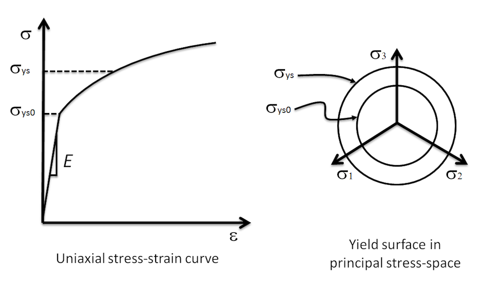
The example material model: Uniaxial stress-strain curve and yield surface in principal stress space.
Now, let’s discuss approaches for implementing a material model as an external material. There are several different ways of calling user-coded routines for external materials, which we refer to as sockets.
Approach 1: General Stress-Strain Relation
We can use the General stress-strain relation socket of the external material to define a complete material model that includes (possibly) both elastic and inelastic strain contributions. This is the most general of the two modeling approaches discussed here. When we use the General stress-strain relation socket, we are faced with two tasks:
- Computation of the stress tensor \bm{\sigma}
- Computation of the Jacobian of stress \bm{\sigma} with respect to strain \bm{\epsilon}
Approach 2: Inelastic Residual Strain
We can also use the Inelastic residual strain socket to define a description of an inelastic strain contribution \bm\epsilon_{inel} to the overall material model. An example of this would be if we wanted to add our own creep strain term to the built-in linear elastic material. The Inelastic residual strain socket assumes an additive decomposition of the total (Green-Lagrange) strain into elastic and inelastic parts. Thus, this is an adequate assumption when strains are of the order < 10%. When we use the Inelastic residual strain socket of the external material model, we are faced with two tasks:
- Computation of the inelastic strain tensor \bm{\epsilon}_{inel}
- Computation of a Jacobian of inelastic strain \bm{\epsilon}_{inel} with respect to strain \bm{\epsilon}
Two related External Material sockets are the General stress-deformation relation and the Inelastic residual deformation. These are more general versions of those discussed above. Instead of defining the deformation in terms of the Green-Lagrange strain tensor, the deformation gradient is provided. Many large-strain elastoplastic material models use a multiplicative decomposition of the deformation gradient into elastic and plastic parts. In these situations, you would likely want to use one of these sockets instead.
Tip: We link to the source file and model file at the bottom of this blog post.
Computation of the Stress Tensor: Stress Update Algorithm
The complexity of computing the stress tensor varies significantly between material models. In practice, the computation of the stress tensor often needs to be formulated as an algorithm. This is often called a stress update algorithm in literature. In essence, the objective of a stress update algorithm for a material model is to compute the stresses, knowing:
- The total strains corresponding to the current estimate of the displacement field
- The material state of the previously converged increment
These quantities are provided to the external material as input.
The term “material state” represents any solution-dependent internal variables that are required to describe the material. Examples of such variables are plastic strain tensor components, current yield stress, back stress tensor components, damage parameters, effective plastic strain, etc. The choice of such state variables will depend on the material model. We must ensure that the material state is properly initialized at the start of the analysis, and that it is updated at the end of the increment.
We first need to investigate if there is plastic flow occurring during the increment. We do this by assuming that the elastic strain is equal to the total strain of the current increment, less the (deviatoric) plastic strain of the previously converged increment, ^{old}\bm\epsilon_{p}. This assumption would hold true if there was, indeed, no plastic flow during the increment. The deviatoric stress tensor that is computed this way is aptly called a trial stress deviator and is given by
with an effective (von Mises) value \sigma_{trial,e}.
The effective trial stress is compared to the yield stress of the material by assuming that there is no plastic flow during the increment. The yield stress corresponding to the previously converged increment is given by
Notice that the left-superscripted ^{old}\bm\epsilon_p and ^{old}\epsilon_{pe} in Steps 1 and 2 represent the material state of the previously converged increment, as we discussed earlier.
Now we check if the trial stress causes plastic flow. For another way of expressing this, if the trial stress is inside the yield surface, the response will be purely elastic during the increment. If not, plastic flow will result. The check is performed using the yield condition:
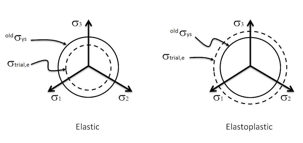
Check of the yield condition to determine elastic or elastoplastic computation.
The stress update algorithm now necessarily branches off into either a purely elastic computation or an elastoplastic computation. We will follow each of these branches, starting with the purely elastic branch.
Elastic Computation
Because we determined that there is no plastic flow during the increment, the trial stress deviator is, in fact, identical to the stress deviator, and the update of the plastic strain tensor and the effective plastic strain is trivial.
We can directly return the pure elastic stress-strain relation as the Jacobian.
Elastoplastic Computation
The objective of the elastoplastic branch of the stress update algorithm is to compute the stress deviator and update the plastic strains. We begin by again expressing the stress deviator, now knowing that plastic flow takes place during the increment:
or
In the above equation, we used a discrete form for the flow rule that states that an increment in plastic strain is proportional to the stress deviator through a so-called plastic multiplier \Delta\lambda. Let’s stop for a moment and consider a graphical representation of this equation for stress:
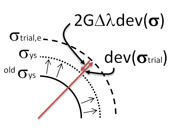
Graphical representation of the correction of the trial stress deviator.
If we compute a trial stress deviator that lies outside the yield surface, we need to make a correction so that the stress deviator is returned to the to-be-determined yield surface. The plastic multiplier determines the exact amount by which the trial stress deviator should be scaled back to give the correct stress deviator. If we compute the plastic multiplier, it is straightforward to then compute the stress deviator and the plastic strain increment.
The key steps are to:
- Transform the equation for stress into a governing scalar equation
- Express all the unknowns in a single parameter
- Solve the scalar equation for this parameter
We can relate the plastic multiplier to the effective plastic strain increment \Delta\epsilon_{pe} using the flow rule and then transform the equation for stress into a governing scalar equation:
This is in general a nonlinear equation, and we need to solve it using a suitable iterative scheme. We are now ready to compute the stress tensor, the plastic strain tensor, and the effective plastic strain.
The updated plastic strain tensor and effective plastic strain are stored as state variables.
Computing the Jacobian of the Material
We computed the stresses and updated the material state (the state variables) for our material model. Now, we turn our attention to the Jacobian computation. The Jacobian has other names in literature, such as tangent stiffness, tangent modulus, or tangent operator. In the stress update algorithm, we express the deviatoric and hydrostatic parts of the stress tensor as:
The Jacobian that we want to compute is the derivative of the Second Piola-Kirchhoff stress tensor with respect to the Green-Lagrange strain tensor. For our example material, we assume that strains are small. This means that we do not need to distinguish between various measures of stresses and strains, because they are indistinguishable in the small-strain limit. The derivative \mathcal{C} of stress with respect to strain is written as
If we use the equations for the deviatoric and hydrostatic stress and the definition of the trial stress, we can express the Jacobian in the following way:
Note that we replaced the increment of the plastic strain tensor by the total plastic strain tensor in the expression above. Their derivatives with respect to strain are the same, by virtue of the additive update of the plastic strains. Recall that our two modeling approaches require differently defined Jacobians. We see immediately how they are related. In the General stress-strain relation, the Jacobian is given by the full expression above. In the Inelastic residual strain, the Jacobian is given by one term in the expression, namely:
The term \mathcal{C}^e is the elastic Jacobian. For a purely elastic computation, the total Jacobian of the General stress-strain relation equals this quantity, while the Jacobian of the Inelastic residual strain in this case is zero.
If we use the flow rule and the chain rule for differentiation, we arrive at the following expression:
Notice that this expression depends on the plastic multiplier. This suggests that for the current material model, there is little benefit in choosing the Inelastic residual strain over the General stress-strain relation, because both approaches require a full stress update algorithm to compute the plastic multiplier. For other material models, such as creep models, the benefit would be greater. Using the governing scalar equation and the flow rule, we can compute the last derivative in the expression above.
In order to ensure rapid convergence of the global equation solver and ultimately reduce the simulation time, the computed Jacobian should be accurate. Well, what does accurate mean? Simply put, it means that the computed derivative must be consistent with the stress update algorithm that was used to compute stresses. That is, any assumptions or simplifications used in the stress update algorithm should be reflected in the computation of the Jacobian. A derivative based on the stress update algorithm is often called algorithmic or consistent.
In some situations, the Jacobian computation can be cumbersome. It is often possible in these situations to use an approximate Jacobian. Keep in mind that the accuracy of the solution is determined by the stress update algorithm. As long as the Jacobian is not too far off, the global equation solver will still converge to the correct solution, albeit at a lower rate of convergence.
Further Comments on Jacobian Computation
- The external material uses a reduced vector and matrix form for stresses, strains, and Jacobians. We need to phrase our stress update algorithm and Jacobian computation accordingly.
- The strain vector that enters into the external material uses tensor components for the shears. The Jacobian is defined assuming tensor components of the shears; therefore, it is generally nonsymmetric.
- The case of plane stress is handled outside the external material feature, so we only need to make one implementation of our model. In other words, the model we implement can be directly used in 3D, 2D axial symmetry, and 2D plane stress and plane strain analyses.
Application Example: Specialization of the Material Model
In the sections above, we developed a stress update algorithm and outlined how to compute a Jacobian. Now, we will consider a special case for the hardening curve. We assume that the yield stress is a linear function of effective plastic strain. This is usually called linear hardening, and it is defined by a constant “plastic modulus” E_{iso}, which is the constant slope of the hardening curve. As it turns out, linear hardening means that the plastic strain increment can be solved on closed form:
In the example’s source code file, we have made use of this specialization into linear hardening.
Let’s consider an example problem of pulling a plate with a hole.
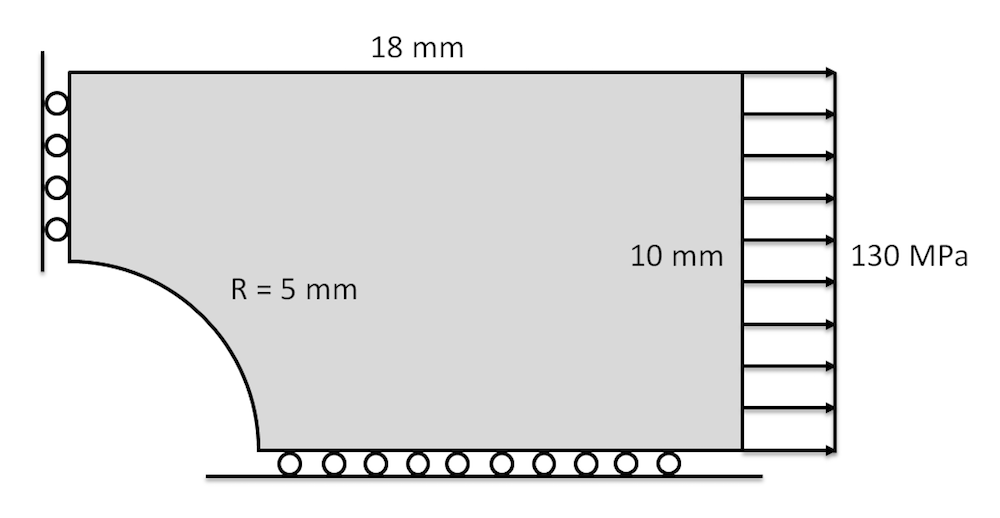
Dimensions, boundary conditions, and loads for a plate with a hole.
The problem has two symmetry planes and only one-quarter of the plate is modeled. We use the following material parameters:
- E = 70 GPa
- ν = 0.2
- \sigma_{ys0} = 243 MPa
- E_{Tiso} = 2.17 GPa
The problem assumes plane stress. We can compare predictions of the implementation of our material model with the built-in counterpart. We expect differences only within the order of numerical round-off as long as the tolerance when solving the nonlinear equations is tight enough.


Computations of the effective von Mises stress in MPa of the external material implementation (left) and built-in material model (right).


Computations of the effective plastic strain for the external material implementation (left) and built-in material model (right).
Some Concluding Remarks
There are actually more scenarios where you can employ the possibility to add external materials.
Consider a situation where you have a source code for a material model that has been verified in another context. You may have created it yourself or found it in a textbook or journal paper. In this case, it may be more efficient to use the external material functionality than casting it into a new form and enter it as set of ODEs. Even when the code is written in, for example, Fortran or C++, it is usually rather straightforward to wrap it into the C interface used by the external material.
A coded implementation may be computationally more efficient than using the User Defined or extra PDE options. The reason is that the detailed knowledge about the material law makes it possible to devise efficient stress updates, using, for example, local time stepping.
Next Steps
- Download the example source code and model files featured in this blog post (linear_hardening.mph, linear_hardening.c, linear_hardening.dll) and get more details on how to use external materials:
- Read a previous blog post about accessing external material models
- Learn more about computational plasticity with these highly informative books:
- J.C. Simo and T.J.R. Hughes, Computational Inelasticity, Interdisciplinary Applied Mathematics, Vol. 7, Springer-Verlag, 1998.
- M. Kojic and K.J. Bathe, Inelastic Analysis of Solids and Structures, Computational Fluid and Solid Mechanics, Springer-Verlag, 2005.
- T. Belytschko, W.K. Liu, and B. Moran, Nonlinear Finite Elements for Continua and Structures, Wiley, 2000.


Comments (36)
Ijaz Shahid
November 11, 2017Respected Professor
I have a question about the elastic-plastic material modeling in COMSOL Multiphysics. Is there is any modeling in COMSOL where i can design my model in elastic plastic region.
Mats Danielsson
November 13, 2017 COMSOL EmployeeHello,
As mentioned in the blog post, there are numerous material models for elasto-plasticity already in the program. If you are interested in modeling the elasto-plastic behavior of a material not already provided, you can use one of the External Material approaches that are discussed in the blog post. To get started, you can download example files using the link under “Next Steps”.
Mats
KAI REN
November 15, 2017Dear Dr. Danielsson,
I have a question about transferring strain fields between two different mph files. Is there a method to transfer strain field in different mph files (when thermal strain, plastic strain are involved), so the later mph file can utilize the result of the former mph file as initial value?
As there exists “initial strain and stress” tag, I wonder how to add initial plastic strain and thermal strain to let comsol distinguish constitution of different strains.
Many thanks,
Kai
Mats Danielsson
November 16, 2017 COMSOL EmployeeDear Kai,
This ia a bit off-topic with regard to the External Material feature, so I suggest that you contact our support.
Mats
hicham CHAOUKI
August 23, 2018Hi Mats,
Thank you for the detailed informations. It is possible to implement the same constitutive law according to the second approach mentioned above (using the PDE tools with weak or strong formulation) ?
Best regards,
H. CHAOUKI
Laval University
Mats Danielsson
August 24, 2018 COMSOL EmployeeHello,
Material models like the one in this blog post use a yield condition. That is why the stress update has to be expressed in terms of an algorithm, where a certain “branch” is traversed depending on the state of the yield condition (elastic vs. elastoplastic). In other words, the elastoplastic behavior cannot be expressed purely in terms of, say, an ODE.
That said, many other material models, such as creep or viscoelastic models, do not feature a yield condition. In these models, inelastic strains are said to develop at every non-zero level of stress, albeit very slowly at low levels. These types of models can be implemented the way you propose.
Mats
Narinder Singh
August 24, 2018Hi Mats,
Thanks for this useful blog. I have a question regarding the total strain increment in the accompanying files.
For calculating trial stress (or strain), shouldn’t the strain increment be equal to e(n+1)-ep(n) ?
Your code writes it as eTrial[i] = e[i] – ep[i], where both e and ep correspond to the current values, making it effectively e(n)-ep(n). Where does the ‘increment’ part come in?
Or if I ask in general, how does one get to access strain increments (for each integration point of each element)? As far I believe, the equation view only shows the current state of quantities.
I am sure I have missed something somewhere. Please clarify.
Thanks
Mats Danielsson
August 24, 2018 COMSOL EmployeeHello,
The trial stress is the stress that is computed assuming that the increment is purely elastic. Therefore it defines a trial strain as the total strain of the current (global) iteration less the total plastic strain of the previous increment. If you look closer at the code, the plastic strains are using values from the states1 array. This states1 array has not yet been updated when the plastic strains are defined, so the values do indeed represent the converged values of the previous increment. If the trial stress violates the yield condition, the code branches off into the elastoplastic part where it computes an increment in plastic strains, and adds it to states1. And so on.
It’s not a strain increment that is used, though. This formulation is total, in the sense that it does NOT use strains from the previous increment to compute an increment in stress. It only uses total strains from the current (global) iteration and the plastic state from the previously converged global increment.
I hope that helps!
Mats
Narinder Singh
August 24, 2018Thanks for the explanation Mats.
I agree with you in principle. Does it mean then that the ‘input’ strains in the code, ‘e’ are the current total strains (effectively, e(n+1)) and not e(n) as I was thinking them to be. In that case, it all makes sense.
Mats Danielsson
August 24, 2018 COMSOL EmployeeHello again.
Yes, the strains that are fed into the code correspond to the current estimate of the displacement field.
Mats
hicham CHAOUKI
September 12, 2018Thanks Mats for all informations. I tried the dll file that I found on website and it works well. However, wen I write my own code and I built up the dll file, Comsol does not work. Could you please give us some informations about the compiler that we need and the methodology to follow.
Best regards,
H. CHAOUKI
Laval University
Mats Danielsson
September 13, 2018 COMSOL EmployeeHello,
With regard to compilation, I suggest you read the section called “How to Compile and Link an External Material Model” in the documentation.
Without more detailed information, it is difficult to know what is going wrong in your particular case. I suggest you contact our support.
Mats
hicham CHAOUKI
October 3, 2018Thank you Mats. Everything is ok with the compilation.
Best Regards,
H. CHAOUKI.
hicham CHAOUKI
November 13, 2018Hi Mats,
I have a question about external material routine for mechanical analysis. I’m working on the developpment of a constitutive law where the mechanical behaviour is coupled with thermal and porous behaviours. The constitutive law depends, among others, on the thermal strain and the pore pressure. I’m wondering if it is possible to pass to the external routine values of the pore pressure and the temperature field and then solve the problem by considering a weak coupling between thermal, mehcanical and porous problems.
Bests regards,
H. CHAOUKI.
Mats Danielsson
November 19, 2018 COMSOL EmployeeHello,
Of course you can pass anything to the external material in the parameter list. With regard to the coupled problem, I advise you to contact COMSOL support as it becomes too complex to address in the blog.
Mats
hicham CHAOUKI
November 19, 2018Hello Mats,
Thank you for the information.
Best regards,
Hicham.
Yu Zhang
January 2, 2019Hi, Mats Danielsson:
Thank you for sharing us this wonderful approach to build our own material model. Now I have a question about the determination of Jacobian matrix. The HELP document mentioned that the Jacobian matrix ” must be provided by the external material functions in the form of partial derivatives of output argument components with respect to input argument components”, as you did in the blog above. However, I found my Jacobian matrix is very difficult to be explicitly expressed as the derivatives of output with respect to input, as you have done in this blog. So I am wondering whether I can express it in an implicit way to achieve the material model.
Any response and help will be highly appreciated.
Yu
Mats Danielsson
January 4, 2019 COMSOL EmployeeHello,
If it is too difficult to express the Jacobian, the first thing to consider is if there are parts of it that you can neglect. Of course, any such departure from the algorithmically consistent Jacobian will affect the rate of convergence, and sometimes to a point of no convergence.
The second thing you can try is to compute a numerical approximation to the Jacobian. You will then use your existing stress update algorithm, together with perturbations to the strain, to compute a numerical Jacobian. A benefit is that you will not need to compute any derivatives apart from what may be required by the stress update algorithm itself. A drawback is that you will execute your stress update algorithm six additional times per stress update.
There is a nice article available on how to do this:
Christian Miehe,
Numerical computation of algorithmic (consistent) tangent moduli in large-strain computational inelasticity,
Computer Methods in Applied Mechanics and Engineering,
Volume 134, Issues 3–4,
1996,
Pages 223-240
Good luck!
Mats
Yu Zhang
January 5, 2019Hi, Mats:
Thank you so much for your valuable and useful reply. May I ask you another question about the compilation of the material model?
The material model I developed contained the utility functions embedded in COMSOL. Thus, I followed the corresponding instructions given in the Users’s Guide. As given in the Guide, the command line in third step is
“link /OUT:Emfracture.dll /DLL Emfracture.obj
C:\Program Files\COMSOL\COMSOL54\Multiphysics\data\extmat\win64\csextutils.lib”
However, I found that the .dll file has already been created after I just input the first line of the contents in the quote. It seems the second line is not necessary. I am not sure whether it is correct without the second line. Would you mind giving me some ideas how to account for the second line in the quote.
Thanks a lot for your time and help.
Yu
Mats Danielsson
January 7, 2019 COMSOL EmployeeHello,
This is slightly off topic, so I suggest you contact support for this.
Mats
Min Mao
December 15, 2019Thank you very much for sharing! Very helpful!
But, where is the linear_hardening.mph ? I did not find this mph file in the link: https://www.comsol.com/model/external-material-examples-structural-mechanics-32331, though linear_hardening.c and linear_hardening.dll are there.
May you please also upload linear_hardening.mph (my version is COMSOL 5.3a) ? Thanks!
Mats Danielsson
December 16, 2019 COMSOL EmployeeHello,
The model files should now be available for the current version (5.5). For an older version, the easiest way is to use the presentation (linear_hardening_V53.pptx) and add the external material definition to your own model file. Slides 8 and 9 show the parameters and states that are required for the example linear_hardening external material.
Mats
Min Mao
December 16, 2019Hi Mats,
Thank you very much for your prompt response and adding the mph file! Unfortunately, my 5.3a version cannot open the mph file of the 5.5 version.
I appreciate your suggestion for the older version, yeah, I have added it into my own model file, and now it works.
Again, thank you so much for your kind help!
Best,
Chao Liang
January 2, 2020Hello,
Thanks for the blog. In the equations you put out, you seemed to have missed a factor of J2 in the plastic follow rule.
If the flow rule is f = \sqrt{3*J2} – \sigma_{Y} = \tau – \sigma_{Y}, classic von Mises. Then the associative flow rule states that \epsilon_{ij}^{p} = \frac{3}{2} \frac{dev(\sigma)}{\sqrt{3 * J2}}.
In your equation, the plastic multiplier \lambda seems to take a the unit of 1/Stress. However, this is not consistent with the later equations you put out, such as the last equation in the section “Computing the Jacobian of the Material”. Could you clarify this? Thanks.
Mats Danielsson
January 7, 2020 COMSOL EmployeeThanks for pointing this out. The expression for the derivative of the plastic multiplier with respect to strain incorrectly included a factor that emerges in the expression for the total Jacobian. This has now been corrected.
With respect to the plastic multiplier, it is simply a scaling between the deviatoric stress tensor and the plastic strain tensor increment.
Mats
Yu Zhang
January 21, 2020Hi, Mats
I have a question about the Jacobian. In your blog, the Jacobian is defined with respect to the INCREMENTAL value of stress tensor and strain tensor. But in the code for “Mazars damage model”, the Jacobian is defined with respect to the TOTAL value of the stress and strain. These are two totally different definations. Does it mean one of the Jacobian is incorrect?
In my model, the stress upstate algorithm is developed by using the incremental stress and strain. So I used the Jacobian between the incremental stress and strain. But the code cannot run, even one step. Which approach as given above should I use to define the Jacobian?
Thank you so much for your help.
Mats Danielsson
January 22, 2020 COMSOL EmployeeHello,
The correct Jacobian is the derivative of total stress (2:nd Piola-Kirchhoff) with respect to total strain (Green-Lagrange). As I wrote in the blog body text, the derivative should be consistent with the stress update algorithm that is being used to compute stresses. This is the Jacobian that is being derived above – using total stresses and total strains.
It is difficult to give a detailed answer to your specific problem, but if your code doesn’t seem to run at all, perhaps the problem is more severe. Make sure that the computations inside the external material work the way you think. But more fundamentally, it would be better to use a total formulation.
Mats
Yu Zhang
January 22, 2020Hi, Mats:
Thank you for your reply. For most of plastic models, the stress update algorithm is developed with respect to the INCREMENTAL strain, i.e. input incremental strain and output incremental stress. Then, the total stress is the sum of the previous converged stress and the calculated incremental stress.
In such case, how to define the Jacobian? It seems more straightforward to define it as: delta_s=Jac*delta_e, where delta_s and delta_e are incremental values in this step. According to your reply, it may be defined as: ds=Jac*de, where ds and de are the derivatives with respect to total value. This definition seems complex, for the stress update algorithm developed by using incremental strain. Could you please give some ideas or share some literature to deal with it?
Thanks a lot.
Mats Danielsson
January 23, 2020 COMSOL EmployeeHello,
Some stress update algorithms work with incremental stresses and strains, and some, like ours, use a total formulation. If you use a stress update algorithm that updates the stress incrementally, you can of course update the stresses this way in the external material. It is often the case that the Jacobian can be approximated with something that is simpler to derive, at the expense of quadratic convergence. In many situations, this is quite acceptable, so I would recommend that you simply try to use the “delta_s = Jac * delta_e” definition to see how it performs. Things to keep in mind are the stress and strain measures that your Jacobian uses. The external material expects a derivative of 2PK stress with respect to GL strain, and if you work with, say, Cauchy or Kirchhoff stresses, you have to convert your Jacobian expression accordingly.
One book, but there are many, that discusses different formulations of the stress update is:
“Nonlinear Finite Elements for Continua and Structures” by Belytschko, Liu and Moran (Wiley).
Mats
Yu Zhang
January 23, 2020Hi, Mats:
I really appreciate your detailed reply. For the stress and strain measures, I think the Jacobian matrix (for 2ed PK stress, Cauchy and Kirchhoff stress) should be the same for the small deformation assumption. Is it correct?
In addition, according to your reply, I think the code for “Mazars damage model” may not be correct, as the Jacobian in the code is: D(d)=(1-d)D_0. I think this definition has missed one term related to the rate of the damage variable. The Jacobian may be D(d)=(1-d)D_0-d(d,TIME)*D_0*e/d(e,TIME). I am not sure my understanding is correct or not. Could you please give some comments on it?
Thanks a lot for your help.
Mats Danielsson
January 24, 2020 COMSOL EmployeeHello.
I suspect that the Jacobian used in the Mazars example is approximate, where terms related to the rate of the damage variable have been neglected, as you indicate.
Mats
Yu Zhang
January 27, 2020Hi, Mats:
The stress update algorithm I used was defined incrementally. I tried the definition of Jacobian, i.e. “delta_s = Jac * delta_e”. However, it seems not correct to define the Jacobian. According to the HELP document, the Jacobian is defined as: ds=Jac*de, where ds and de are the derivatives with respect to total value. However, for the incremental stress update algorithm, this Jacobian definition seems difficult to be determined. It may be calculated as: d(s_pre+delta_s)=Jac*d(e_pre+delta_e), where _pre means the value at previous converged step. As the s_pre and e_pre are constants at current step, this defination can be simplified as: d(delta_s)=Jac*d(delta_e), which is similar to the first one, i.e. “delta_s = Jac * delta_e”. So I am wondering how to determine the correct Jacobian based on the definition: ds=Jac*de, if the stress updated algorithm is defined incrementally?
Thanks for your help.
Yu Zhang
January 22, 2020Hi, Chao:
It seems that the coefficient from the associative flow rule has been lumped into delta_lamd, as seen in the code.
Sidi Mohammed Daoud
December 16, 2020Hello, Professor
I want to model an experiment that consists of loading a non-coherent soil by a prescribed displacement.
The soil characteristics are:
– Young’s modulus: 10 MPa
– Poisson’s ratio: 0.26
– Internal angle of friction: 39 deg
– Cohesion: 0 (for convergence reason, I took c=1Pa)
The imposed displacement is 20mm (I used the auxiliary sweep option)
the software displays the message:
Failed to find a solution for all parameters, even when using the minimum parameter step.
Failed to compute elastoplastic strain variables.
Returned solution is not converged.
I tried all the recommendations given in the Comsol website.
James Smith
August 3, 2024Can I transfer dependent variables from other physical field interfaces into external materials for calculations? For example, I want to perform coupled calculations at the dilute matter transfer interface and the solid mechanics interface, where matter concentration affects the intrinsic behavior of the material, and material deformation affects matter transport. I understand that modifying the weak form of the equations at the corresponding interface can easily achieve this purpose.
However, if I use an external material under the solid mechanics interface, how should I implement it to enable the input and output of the dependent variable from the dilute matter transfer interface in the external material? Is this process currently feasible? If so, how should it be accomplished?
Mats Danielsson
August 5, 2024 COMSOL EmployeeHello.
You can always pass information to and from the external material using the states array. However, some Jacobian contributions from the coupling of the fields will be missing as the external material only considers the d(stress)/d(strain) part. Whether this is sufficient for your purposes, I don’t know.
Mats