
When setting up fluid flow simulations, we typically focus on a single (possibly a few) components in a larger system, such as a pump or sedimentation tank in a water treatment plant. Naturally, this raises a question: At what distance can we apply boundary conditions without interfering with the process? In this blog post, we look at the effects of the proximity of inlet and outlet boundaries for interior and exterior flows of a homogeneous fluid with negligible compressibility.
Placing Inlet and Outlet Boundaries for Interior Flow
CFD simulations are usually computationally demanding and we naturally try to minimize the degrees of freedom in our simulations. If we take it to the extreme, we might end up with a geometry in which an inlet boundary and an outlet boundary intersect. Let’s consider a sharp 90° bend in a pipe with a semicircular cross section.
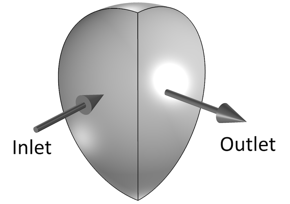
A pipe with a 90° bend and semicircular cross section.
If the simulation is set up using the geometry shown above, the inlet and outlet boundaries share an edge. In many cases, this issue alone may cause severe convergence problems. However, in this particular case, the solution converges within a few iterations. We also consider an appropriately set up simulation with inlet and outlet pipes extended to a length of 10 radii (shown below).
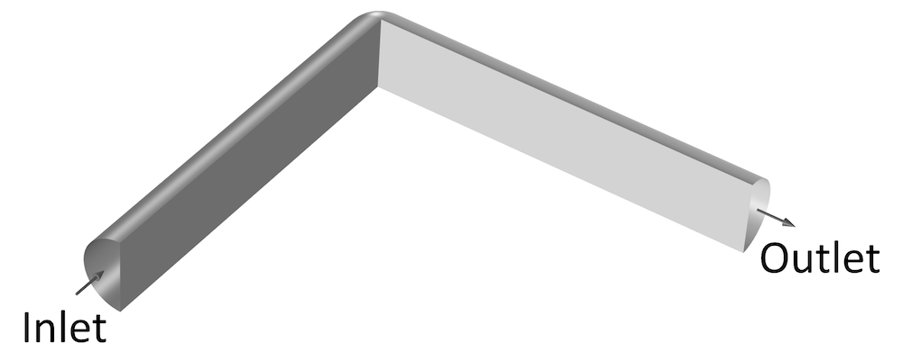
A 90° bend with extended inlet and outlet pipes.
The simulations are performed for a Reynolds number of 120, based on the hydraulic diameter, D_{h}=4A/P, where A is the area of the cross section and P is its perimeter. A uniform velocity profile is applied at the inlets and 0 normal stress is applied at the outlets. The image below shows the pressure at the bend for the two simulations, with extended inlet and outlet pipes on the left and without these pipes on the right. For the case with extended inlet and outlet pipes, the average pressure on the downstream boundary is subtracted from the pressure in order for both results to have 0 average pressure on this boundary.
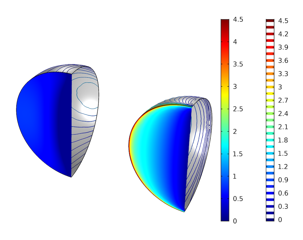
Pressure variation across a 90° bend in a pipe with a semicircular cross section, with pressure surface plots on the upstream boundary and pressure contours on the pipe walls. The left plot shows the results with extended inlet and outlet pipes and the right plot shows the results without these pipes.
The results from the simulation without extended inlet and outlet pipes show a much larger pressure variation. There is a sharp pressure gradient at the wall next to the inlet due to the incompatibility between the applied uniform velocity profile and the No Slip boundary condition at the wall. The plot to the left shows a much more uniform pressure on the upstream side of the bend, which indicates that the flow is fully developed when it reaches the bend. The pressure is not entirely uniform, though: It appears slightly lower close to the sharp corner. This indicates an upstream influence of the bend. We also see a stagnation point on the pipe wall opposite to the upstream boundary. The loss coefficient across the bend, defined as
(1)
is 2.3 without the extended inlet and outlet pipes and 0.60 with them. More insight can be gained by looking at the velocity field.
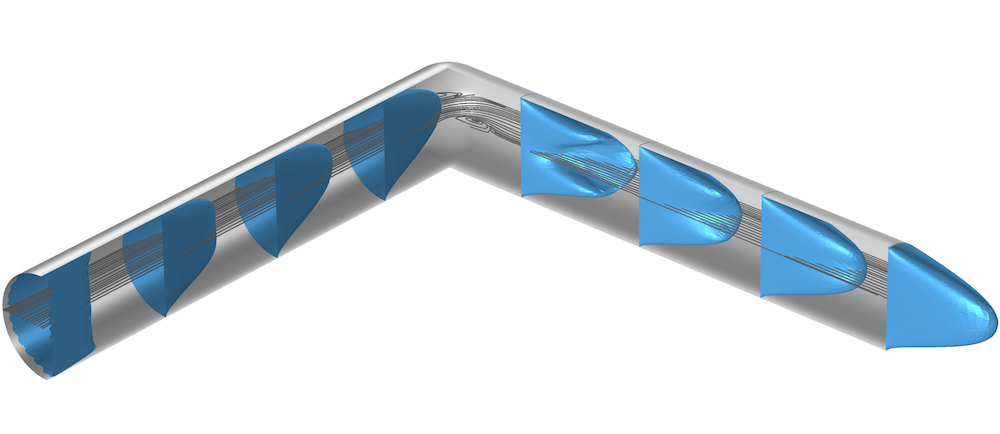
Velocity profiles and streamlines in a 90° bend for a pipe with a semicircular cross section.
The figure above shows the velocity profile at four positions upstream of the bend and four positions downstream of the bend as well as the streamlines in the center plane. Upstream, we can see how the uniform velocity profile evolves into the fully developed profile. At the bend, we see the stagnation point on the pipe wall facing the inlet pipe and the associated recirculation zone. Downstream of the sharp bend, there is another recirculation zone, and we can see that the fully developed profile is obtained first at the end of the outlet pipe. All of this is absent in the simple geometry (containing only the 90° bend), and it is not surprising that we get an erroneous pressure drop.
The Fully developed flow option in the Inlet and Outlet boundary features can be used to avoid excessively long inlet and outlet pipes. The results in the two previous figures strongly indicate that we should apply these conditions at some distance from the bend to obtain good results. But how far upstream and downstream do we need to apply the Fully developed flow options? If we extend the inlet and outlet pipes 1 radius each from the bend, the resulting loss coefficient across the bend becomes 0.54, whereas 2 radii in each direction results in a loss coefficient of 0.58. From there on, the convergence toward the value 0.60 is slower. Hence, 2 radii in each direction seems to be a good trade-off in this case.
As the Reynolds number increases, the recirculation zone downstream of the bend will increase in length and eventually become unstable. For a Reynolds number of 1200, the loss coefficient does not change appreciably when extending the outlet pipe beyond 20 radii, provided that the Fully developed flow option is applied at the end of the pipe. From correlations for entrance lengths in pipes,
(2)
for laminar flow and
(3)
for turbulent flow, we can estimate how far downstream the bend the fully developed flow profile is obtained. Note that the turbulent flow entrance length is usually shorter than the high-Reynolds-number laminar flow entrance length. We have to go to Reynolds numbers of O(10^8) for the entrance length to reach O(10^2) hydraulic diameters.
For the two laminar cases with Reynolds numbers of 120 and 1200, the entrance lengths obtained from (2) are about 7.5 and 75 radii, respectively. By using the Fully developed flow option at the outlets, we obtain good results with outlet pipes corresponding to 1/3 of these lengths.
As for the upstream influence, it should reduce with increasing Reynolds numbers, as the elliptic nature of the Navier-Stokes equation diminishes with increasing Reynolds numbers. We can estimate the region of upstream influence by looking at the potential flow in a similar geometry.


Mapping the upper half plane to a sharp 90° bend using the Schwarz-Christoffel transformation.
Using the Schwarz-Christoffel transformation (Ref. 1), the upper half plane in the complex z-plane can be mapped onto a sharp 90° bend in the complex \zeta-plane. The inlet, located at -i\infty in the \zeta-plane, corresponds to a source at the origin in the z-plane, whereas the outlet is located at \infty in both planes. The outer and inner corners of the bend in the \zeta-plane correspond to the points -1 and 1, respectively, in the z-plane. The velocity field in the \zeta-plane is obtained on implicit form as
(4)
The image below shows the pressure coefficient along the inner wall as a function of the dimensionless distance upstream of the bend for the potential flow solution.
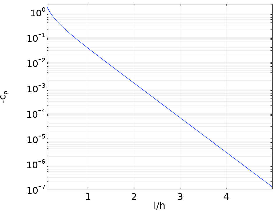
The pressure coefficient along the inner wall upstream of a sharp 90° bend.
In the figure, the pressure coefficient is based on the difference between the local pressure and the pressure far upstream and h is the channel width. We observe that the pressure coefficient is O(10^{-3}) when the upstream distance to the bend is two channel widths. Hence, provided that we use the Fully developed flow option at the inlet, we only need to extend our inlet pipe (or channel) a couple of hydraulic diameters upstream.
Accounting for Gravity
The Fully developed flow option in the Inlet and Outlet boundary features comes with the additional Compensate for hydrostatic pressure option (incompressible flow) or Compensate for hydrostatic pressure approximation option (weakly compressible or compressible flow) when gravity is active in the model. This additional option gives the exact hydrostatic pressure profile on the boundary for incompressible flow and a good approximation for weakly compressible flow and compressible flow. Extra care has to be taken when the fluid at the inlet or outlet boundary is strongly stratified, such as in multiphase flow. In these cases, it might be worthwhile to add a chamber where the flow is made parallel to the gravity vector.
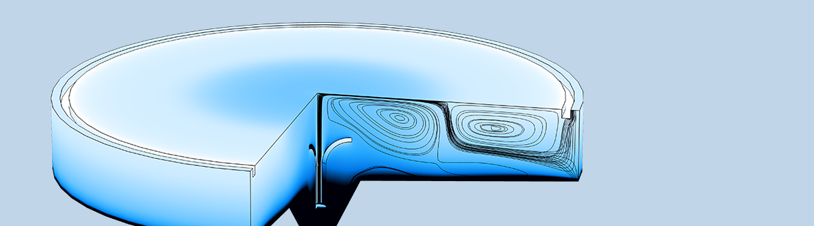
Problems may also arise when working against gravity. The image below shows a large sedimentation tank with a long residence time, allowing the suspended (heavy) phase to settle and exit through the bottom outlet. The light phase exits vertically through an annular outlet located next to the outer rim. The gray streamlines correspond to the velocity field for the light phase, whereas the black streamlines correspond to the velocity field for the heavy phase. A small part of the heavy phase exits through the light-phase outlet. Here, the heavy phase flows in the direction opposite to gravity, causing a small vortex to form next to the outer rim as some of the suspended particles fall back down again. This small vortex can have a negative impact on the time step, resulting in a longer total computational time. A remedy might be to add an overflow (a weir), allowing the flow to exit in the direction of gravity.
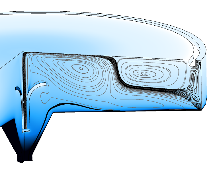
Volume fraction of the dispersed phase (color map) and streamlines, gray for the light phase and black for the heavy phase, in a sedimentation tank.
Another example of a case where inflow and outflow boundaries intersect occurs when simulating a thermal plume, displayed below. In this case, an Inlet boundary condition is not prescribed at the inflow boundary (the cylindrical surface in the figure). Instead, the Open Boundary feature is applied. In both the Open Boundary feature and the Outlet feature (top boundary), the Compensate for hydrostatic pressure approximation option is applied. This is essential since the buoyancy-induced pressure in the model is three orders of magnitude smaller than the hydrostatic pressure. Another option that is also essential is the Suppress backflow option in the Outlet feature.
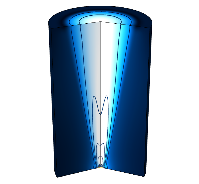
Turbulent thermal plume, showing the velocity magnitude (color map) and contours of the pressure deviations from hydrostatic conditions.
The small perturbations of the contour lines at the top boundary are due to the inconsistency with a constant pressure. These can be eliminated by using the Boussinesq approximation option in the Nonisothermal Flow multiphysics coupling node.
Placing Inlet and Outlet Boundaries for Exterior Flow
In exterior flow applications, such as flow around vehicles and buildings, the conditions far away from the obstacle are usually set to a constant velocity vector on inlet boundaries and a constant pressure on outlet boundaries. The question again arises as to what extent the distance from the obstacle at which these conditions are applied influences the solution. For exterior flow, it turns out that this distance varies with the spatial dimensions of the model. For 2D models, the required distance is an order of magnitude larger than for 3D and 2D axisymmetric models. Once more, we look at ideal potential flow solutions to try to understand why this is so.
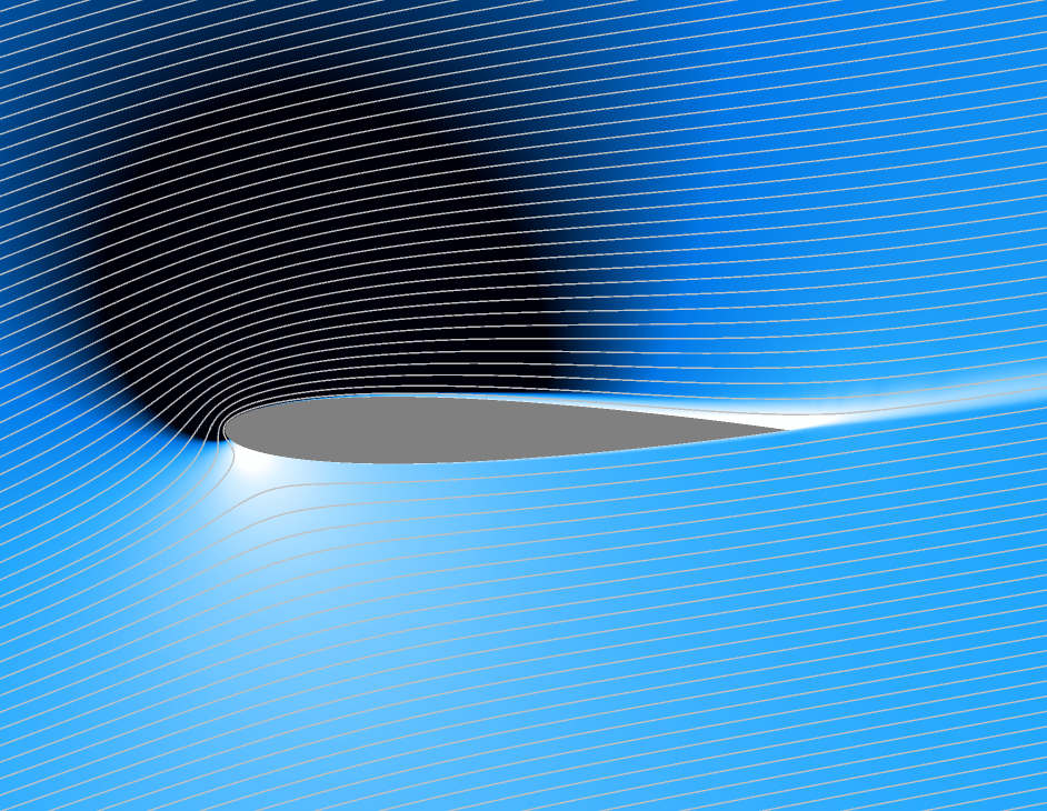
For exterior flow around an obstacle, vorticity is created in boundary layers on the solid surface. The boundary layers on different sides of the obstacle may merge at the trailing edge, forming a thin sheet of vorticity that is advected downstream into a wake. If the boundary layer on any side separates from the obstacle due to an instability or the existence of a sharp convex corner, the wake will be wider. In either case, the vorticity that is shed downstream is confined to the wake and the flow outside the wake is approximately irrotational.
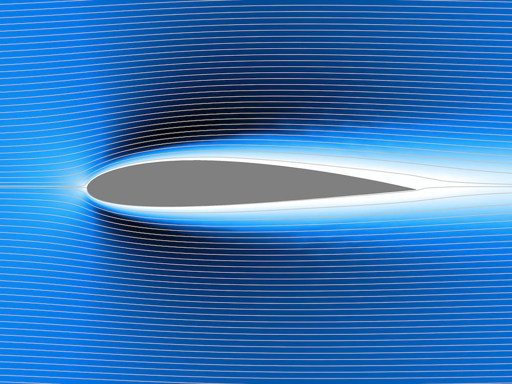
Turbulent flow around a NACA airfoil. The boundary layer on the upper side of the profile separates ahead of the trailing edge.
The obstacle and its wake displaces the streamlines of the free stream, and we may think of the flow at large distances from the obstacle as being the sum of a uniform flow and a source.
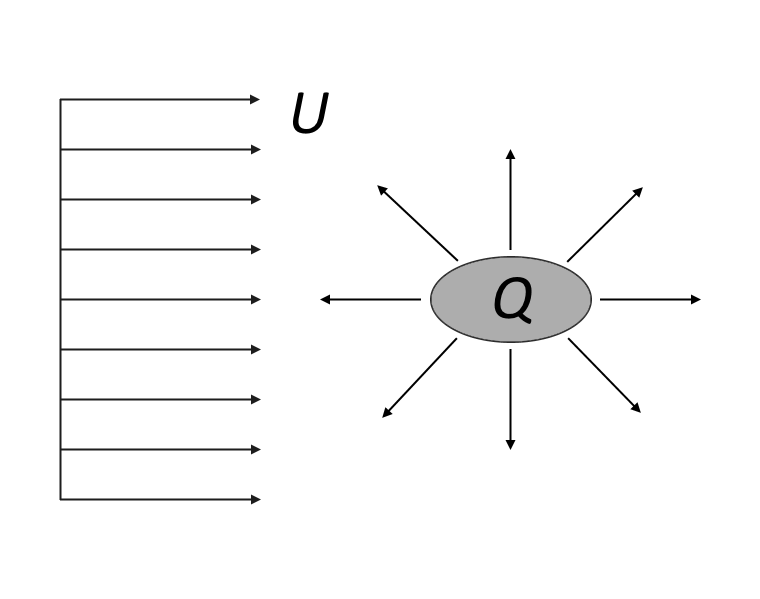
Potential flow at large distances from an obstacle and its wake.
The resulting velocity fields in 2D and 3D can be expressed as
(5)
(u,\, v)&=(U+\frac{Qx}{2\pi R^{2}},\, \frac{Qy}{2\pi R^{2}}),\hspace{12mm}\text{in 2D}\\
(u,\, v,\, w)&=(U+\frac{Qx}{4\pi r^{3}}, \,\frac{Qy}{4\pi r^{3}}, \,\frac{Qz}{4\pi r^{3}}), \hspace{5mm}\text{in 3D}
\end{align}
where R=\sqrt{x^{2}+y^{2}}, r=\sqrt{x^2+y^2+z^2}, the source is located at the origin, and the free-stream flow is directed in the positive x direction.
The source strength can, in either case, be related to the dimensions of the obstacle. At the x-position of the source, the displacement of the streamlines is y_{0}=Q/(4U) in the 2D case and r_{0}=\sqrt{Q/(2\pi U)} in the 3D case. The limiting values far downstream are y_{\infty}=Q/(2U) and r_\infty=\sqrt{Q/(\pi U)}, respectively. For the purpose of the current estimates, either 2y_{0} or 2y_\infty in 2D and 2r_{0} or 2r_\infty in 3D may be used as a representative value for the size of the obstacle. Here, we use d=Q/(2U) in 2D and d=\sqrt{2Q/(\pi U)} in 3D. From Bernoulli’s equation, we get an estimate of the pressure coefficient at large distances
(6)
Inserting the potential flow velocity fields together with the estimates for the source strengths, we find
(7)
c_p&=-\frac{2}{\pi}\left(\frac{x}{R}\right)\frac{d}{R}+O\left(\left(\frac{d}{R}\right)^2\right) \hspace{5mm}\text{in 2D}\\
c_p&=-\frac{1}{4}\left(\frac{x}{r}\right)\frac{d^2}{r^2}+O\left(\left(\frac{d}{r}\right)^4\right) \hspace{6.2mm}\text{in 3D}
\end{align}
Hence, the pressure coefficient diminishes as d/R in 2D and as (d/r)^2 in 3D. To reduce the influence of the exterior boundary conditions to say O(10^{-2}), we would have to locate the exterior boundaries of the computational domain a distance of order of 100 obstacle sizes away in 2D and 10 obstacle sizes away in 3D.
Depending on the shape and orientation of the obstacle, the vortex shedding may induce a circulation that creates side forces (lift). The potential flow at large distances from the obstacle may be approximated by a uniform flow and a point vortex in 2D or a uniform flow and a horseshoe-shaped line vortex in 3D.


Potential flow around an obstacle with circulation (lift). In 2D (left), the potential flow consists of a uniform flow in the x direction and a point vortex located at the origin. In 3D (right), the potential flow consists of a uniform flow in the x direction and a horseshoe vortex with span s in the z direction and extending to infinity in the x direction.
At large distances from the obstacle, the potential flow velocity fields corresponding to the figure above are given by
(8)
(u,\,v)& = (U+\frac{\Gamma y}{2\pi R^2},\,-\frac{\Gamma x}{2\pi R^2}),\hspace{134.4mm}\text{in 2D}\\
(u,\,v,\,w)& = (U+\frac{\Gamma y}{4\pi R^2}\left(\frac{z+s/2}{\sqrt{R^2+(z+s/2)^2}}-\frac{z-s/2}{\sqrt{R^2+(z-s/2)^2}}\right),\,-\frac{\Gamma x}{4\pi R^2}\left(\frac{z+s/2}{\sqrt{R^2+(z+s/2)^2}}-\frac{z-s/2}{\sqrt{R^2+(z-s/2)^2}}\right) \\
& -\frac{\Gamma (z+s/2)}{4\pi (y^2+(z+s/2)^2)}\left(1+\frac{x}{\sqrt{R^2+(z+s/2)^{2}}}\right)+\frac{\Gamma (z-s/2)}{4\pi (y^2+(z-s/2)^2)}\left(1+\frac{x}{\sqrt{R^2+(z-s/2)^{2}}}\right), \\
& \frac{\Gamma y}{4\pi (y^2+(z+s/2)^2)}\left(1+\frac{x}{\sqrt{R^2+(z+s/2)^{2}}}\right)-\frac{\Gamma y}{4\pi (y^2+(z-s/2)^2)}\left(1+\frac{x}{\sqrt{R^2+(z-s/2)^{2}}}\right)),\hspace{7mm}\text{in 3D} \\
\end{align}
Note that the 2D solution is obtained from the 3D solution by setting z to zero and letting s\rightarrow\infty. The circulation can, in most realizable cases, be related to the free-stream velocity and the streamwise dimension (chord) c , of the obstacle by
(9)
where \alpha is the angle of attack and -\beta is the “zero lift” angle (both in radians).
The latter results from the shape (curvature) of the obstacle; an airfoil camber, for example. Inserting the asymptotic potential flow solutions and the expression for \Gamma into the definition of the pressure coefficient, we obtain
(10)
c_p&=-\left(\frac{y}{R}\right)\frac{c}{R}(\alpha+\beta)+O\left(\left(\frac{c}{R}(\alpha+\beta)\right)^2\right) \hspace{13.5mm}\text{in 2D}\\
c_p&=-\frac{1}{2}\left(\frac{y}{R}\right)\frac{s}{R}\frac{c}{R}(\alpha+\beta)+O\left(\left(\frac{s}{R}\frac{c}{R}(\alpha+\beta)\right)^2\right) \hspace{5mm}\text{in 3D}
\end{align}
The total deflection angle, \alpha+\beta, must be at least one order of magnitude smaller than unity so that the estimate for \Gamma holds. For a sphere, the dimensions d, c, and s are equal. Hence, the restrictions on the proximity of the outer boundaries set by the circulation are less severe than those set by the source.
For an airfoil, the three dimensions are all of different orders of magnitude s\sim 10c\sim 100d. In 2D, the restrictions posed by the point vortex are of equal size to those posed by the source, since d\sim c(\alpha+\beta). If a 3D airfoil were to be modeled on its own, the restrictions posed by the line vortex would be a factor of 100 times more severe than those posed by the source. Often, the airfoil is attached to a fuselage with d\sim c, in which case both restrictions become of equal order in the 3D case. The image below shows a 2D simulation of the flow around a NACA 0012 airfoil at a 14° angle of attack. To minimize the influence of the exterior boundary conditions, the domain is extended 100 chord lengths in each direction. The relevant length scale in this case is c\alpha, as \beta=0 for a symmetric profile. According to the above estimates, this results in pressure coefficients of a few tenths of a percent.
2D simulation of a NACA 0012 airfoil at a 14° angle of attack.
The figure below shows a 3D simulation of a stalling airplane at a 20° angle of attack. The computational domain is bounded by a half sphere with a radius of 15 m and a cylinder with a height of 30 m. The wing span is about 18 m, the diameter of the fuselage is 2.4 m, and the maximum chord times the angle of attack is about 1.3 m. Plugging in these numbers results in pressure coefficients of a few percent, which is a bit high. Hence, the results of this simulation would likely improve if the domain was extended farther away from the airplane.
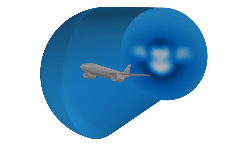
Computational domain, colored by velocity magnitude, for the simulation of a stalling airplane.
Concluding Thoughts on Positioning Inlet and Outlet Boundary Conditions
In this blog post, we demonstrated the use of ideal flow theory and empirical correlations to determine appropriate locations for inflow and outflow boundaries. For interior flow, we used empirical correlations for laminar and turbulent flow to determine the pipe length required to obtain fully developed flow. Extending the domain upstream and downstream accordingly clearly resulted in accurate flow simulations. However, this length increases with the Reynolds number and can, especially for high-Reynolds-number laminar flows, become excessive. Using the Fully developed flow options in the Inlet and Outlet boundary features substantially reduces this length. On the downstream side, a reduction of the length by a factor of three seems to be a decent trade-off between accuracy and computational cost. Using potential flow theory shows that the upstream distance needs to be no longer than a couple of hydraulic diameters. The Fully developed flow option also takes gravity into account when it is active. Problems may still occur when the flow is strongly stratified, such as in multiphase flow. In such cases, it is advisable to redirect the outlet in the direction of gravity.
For exterior flow, potential flow theory was used to estimate the distance at which pressure variations induced by the flow around an obstacle become negligible. It was found that the pressure varies according to \sim D/R in 2D and according to \sim A/R^2 in 3D and 2D axisymmetry, where R is the distance to the center of the obstacle while D and A are the length and area of the obstacle projected onto a plane orthogonal to the free stream, respectively.
Hopefully, these estimates will be useful when you set up your own simulations. Remember to check your results, though. When using the Fully developed flow option for interior flow, the easiest way is to vary the inlet and outlet channel or pipe lengths to see if the results change. For exterior flow, check that the velocity doesn’t deviate by more than the allowed tolerance from the free-stream velocity field on pressure boundaries, except for in the wake, and similarly for the pressure on velocity boundaries.
Reference
- R.V. Churchill & J.W. Brown, Complex Variables and Applications, 5th ed., McGraw Hill, 1990.
Editor’s note: This blog post was updated on 4/25/2023 to reflect that the Fully developed flow option is part of the COMSOL Multiphysics® platform product.

Comments (7)
Saeid Kheirandish
May 3, 2022Thanks for the introduction. Could you please make a remark about the BCs for laminar flow of a highly viscous or non-Newtonian fluid into air (exit flow of polymer melt from a channel)?
Mats Nigam
May 4, 2022 COMSOL EmployeeDear Saeid,
I would include part of the upstream channel and (if applicable) use the fully-developed-flow option. You could check out some of the models in the Application Library for the Polymer Flow module: 2D Non-Newtonian Slot Die Coating, Rubber Injection Molding and Slot Die Coating With Channel Defect.
Best regards,
Mats
Santhosh Babu Mamidala
October 26, 2022I have doubt regarding inlet BC. I have 3D flow case where there is inlet flow which is blasius boundary layer and interacting with a wall-normal jet at some downstream distance. Is there a way to specify the inlet BC to be a velocity profile?
Mats Nigam
October 26, 2022 COMSOL EmployeeDear Santhosh,
In the settings window for the inlet condition, you can select “Velocity field” and type in any expression for each of the velocity components.
Santhosh Babu Mamidala
October 27, 2022Thanks a lot. I understand.
Nguyen Camlai
July 20, 2023Thank you Mats Nigam.
Could you please help me, if in my case the fluid is pressed at high pressure of 30MPa and then flows into a pipe. How do I set the inlet and outlet pressure for the pipe? Or do you know how to set the BCs?
Mats Nigam
July 31, 2023 COMSOL EmployeeDear Nguyen,
It’s hard to say anything specific without more details about the geometry and flow conditions. Are the inlet and outlet connected to pressurized chambers which are held at constant pressure levels, and if so, are these domains part of your model? Is the flow compressible? If you have a model that you need help with, you can send it to our support team.
Best regards,
Mats