
Today, we invite guest blogger F. Xavier Alvarez of Universitat Autònoma de Barcelona (UAB) to discuss modeling heat transfer at the nanoscale using a novel theoretical framework and the COMSOL Multiphysics® software.
The electronics industry develops increasingly smaller electronic devices, which generate heat that needs to be dissipated. The observed evidence is that at shorter scales, heat is more difficult to extract than what Fourier’s law predicts, suggesting its limited validity. Our current research focus is solving this open problem.
Using Fourier’s Law to Describe Heat Transport
In 1822, Fourier published Théorie Analytique de la Chaleur (Analytical Theory of Heat). Since then, Fourier’s law has been successfully used to describe a lot of different experimental observations in a large variety of systems — with remarkable results. Fourier’s law is described by a simple relation between the thermal gradient and the heat flux:
(1)
where \lambda is the thermal conductivity, a property of the material.
In the past few decades, evidence has suggested that Eq. (1) is not correct in the analysis of devices with characteristic lengths L smaller than the mean free path of the heat carriers (phonons). The observed heat flow becomes much smaller than that predicted by Fourier’s law, worsening the capacity of these components to release the excess heat. This issue is usually solved by using an effective thermal conductivity depending on the characteristic length \lambda (L), which has to be empirically determined.
Kinetic theory allows us to obtain correct prediction of thermal conductivity in simple geometries, but its application is not feasible at present in the complex geometry of an electronic device.
Introducing the Kinetic-Collective Model for Hydrodynamic Thermal Transport
The kinetic-collective model (KCM), developed at UAB, is a theoretical framework focused on describing heat transport at the nano- and microscales, as well as calculating the corresponding transport parameters that appear in the equations from microscopic calculations. It is only by this combination of computations that we are able to get a predictive model.
The first-order correction to Fourier’s law is the Guyer–Krumhansl equation:
(2)
This equation is combined with a boundary condition for the flux. For pedagogical reasons, we use the simplest version here:
(3)
Notice that the new Laplacian term in Eq. (2) changes Fourier’s law into a law resembling Stokes equation for a viscous fluid. For this reason, the behavior following Eq. (2) is usually called phonon hydrodynamics. The new term introduces a heat viscosity that reduces the effective conductivity in regions where the flux is not homogeneous. In these regions, the heat flux and the temperature gradient will not be parallel anymore, which has important consequences for the heat and temperature distributions.
It is useful to analyze the different consequences of Eq. (1) and Eqs. (2–3) using a simple geometry like a nanowire. In the image below, we can see the heat flow inside a nanowire with a radius of 500 nm that is heated on one end and cooled on the other. Hot and cold temperatures are imposed on the opposite ends of the wire and periodic conditions are used for the flux to avoid boundary effects on the profile. The temperature profile is the same in all of the cases: a constant gradient in the longitudinal direction with no variation in the transverse direction. The flux is plotted for a range of situations with an increasing value of viscosity, starting from Fourier’s law (l=0) to a value of l = 300 nm. The main difference can be easily observed: While Eq. (1) gives a constant flux on the cross section, Eqs. (2–3) give a curved flow profile.
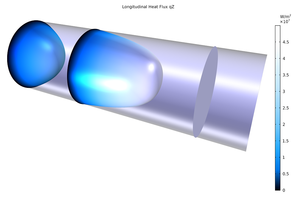
Longitudinal heat flux inside a nanowire with a radius of 500 nm. The three slides show the heat flux profile obtained from Eqs. (2–3). The flat profile corresponds to l=0 (equivalent to Fourier’s law), the medium one to l=100 nm, and the left one to l = 300 nm. The total heat flux decreases with increasing l, leading to a reduced effective conductivity of the nanowire.
Curvature of the heat flux appears because the effect of the boundary reduces the flow in a region of width l. When l is small in comparison with the radius of the wire (l<R), the flow is shown to be affected only in a cylindrical crust near the boundary, called the Knudsen layer. Outside this layer, the value of the heat flow corresponding to the Fourier limit is recovered.
When the characteristic length is of the same order as the wire’s radius, the Knudsen layer increases until the effects are also noticed at the center. At this point, the flow is reduced everywhere in the cross section of the sample and the flow profile shows similarities with the parabolic Poiseuille flow for viscous fluids.
As we pointed out previously, the most important aspect of determining the thermal transport equation in nanowires is that it is not possible to experimentally obtain the profile of the heat flux within the cross section. The only magnitude that can be measured is the effective thermal conductivity, defined as the averaged flux over the cross section divided by the gradient of temperature. This prevents us from experimentally distinguishing if we are observing a behavior predicted from the Guyer–Krumhansl equation or simply a behavior from Eq. (1) with the reduced effective thermal conductivity.
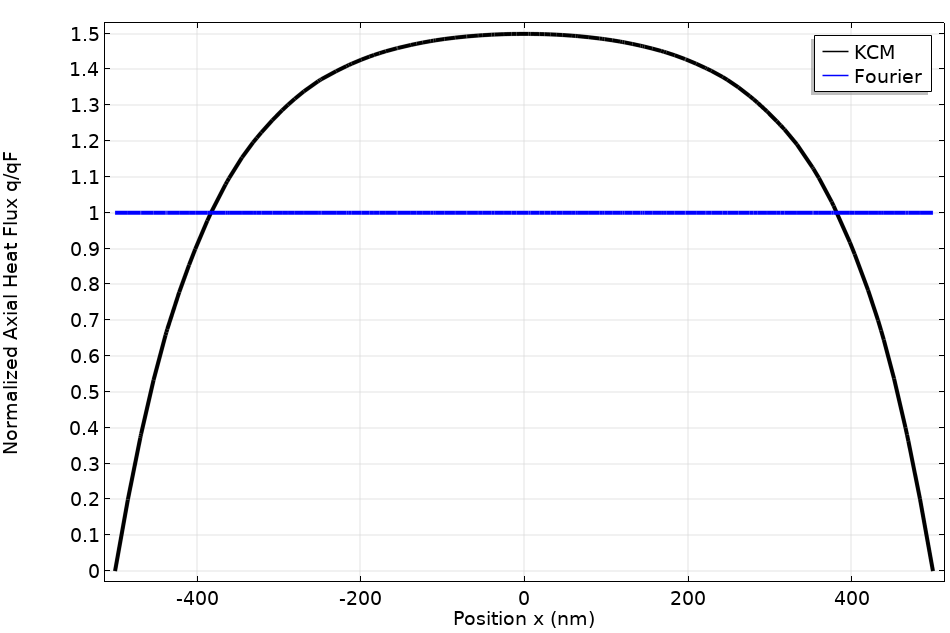
Flux profiles across a wire diameter using the KCM (black line) with l = 100 nm and Fourier’s law (blue line).
The plot above shows two different flux profiles across a wire diameter. The black line is the result when using the KCM with a nonlocal length of 100 nm and the blue line is the Fourier profile. Both systems have the same effective thermal conductivity because their average fluxes are the same. Consequently, they give the same experimental result.
To determine if this equation is valid, a spatially resolved measure is necessary. This has recently been done using a thermoreflectance setup.
Measuring the Thermoreflectance of a Semiconductor Substrate in COMSOL Multiphysics®
Reflectivity is the material property that indicates the ability of a surface to reflect an electromagnetic wave. One important characteristic of this magnitude is that it is temperature dependent. This allows thermoreflectance imaging (TRI) measurements, in which the light reflected by the surface is used to obtain its temperature.
The Birck Nanotechnology Center (BNC) at Purdue University recently developed a thermoreflectance setup and measured the temperature of a silicon substrate when heat is released from metallic lines of different submicrometric lengths on the top. The results can be observed below.
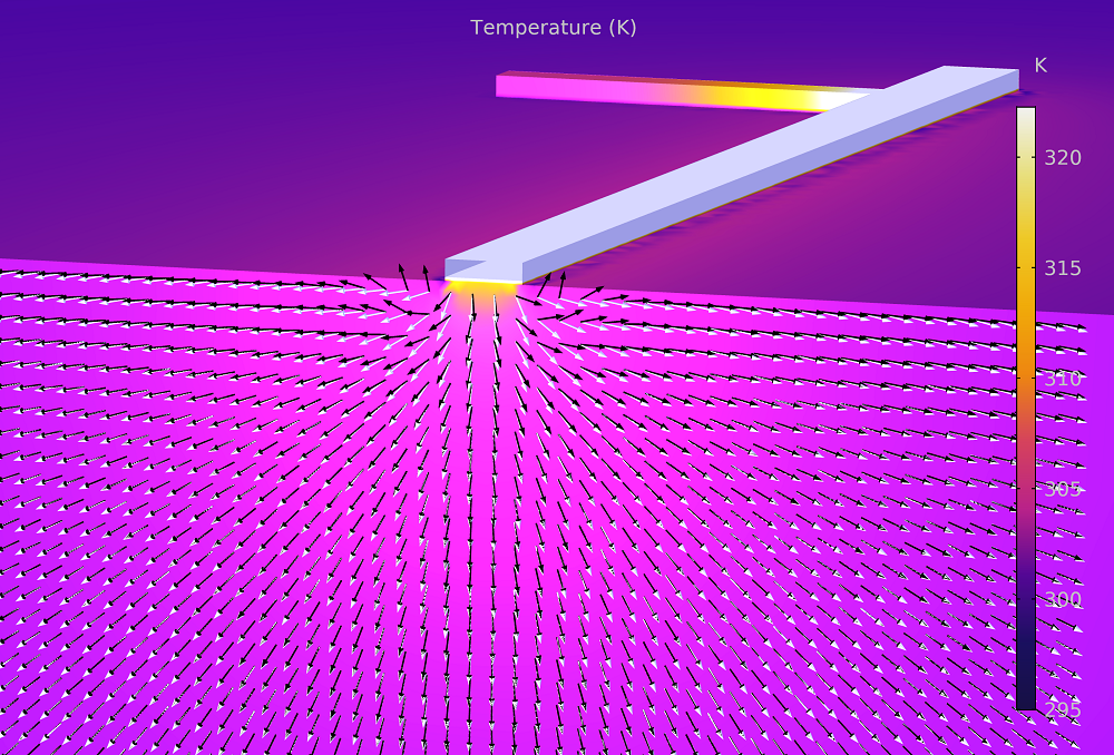
Directions of the heat flux (white arrows) and the temperature gradient (black arrows) in a silicon substrate heated from a submicrometric metallic line obtained using the KCM. Near the line, the heat viscosity is important, which is revealed by the fact that the heat flux and the temperature gradient vectors do not have the same direction.
The question that the BNC and UAB groups have tried to solve is whether the experiment can be described by the use of an effective Fourier’s law or if we need to use an improved model. The complexity in the geometry is significantly higher than in the previous case, so it is important to have a tool that can solve the thermal behavior in this situation. This is where the combination of the simplicity of the KCM theoretical approach and the power of the finite element solver in COMSOL Multiphysics come together.
COMSOL Multiphysics allows us to completely define the experiment, including consistency in the substrate, an insulation layer of oxide, and the metallic line at the top. Contrary to the Boltzmann transport equation approach, these simple equations can be easily solved in a full 3D model.
It can be observed that Fourier’s law is not able to describe the full set of data with the nominal value, or a fitted or effective value, for the thermal conductivity.
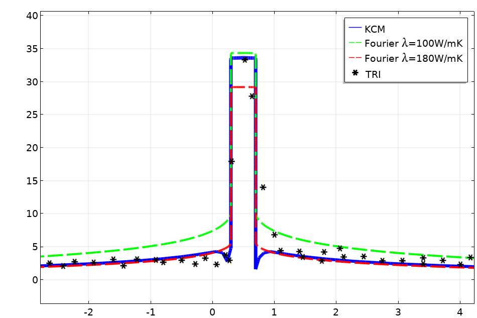
A plot of the temperature profile obtained from the thermoreflectance imaging (TRI) measurement (asterisks) compared with the prediction obtained from Fourier’s law with an increased value of the conductivity (red line), Fourier’s law with a conductivity reduced to fit the heater temperature (green), and the KCM (blue).
In the plot above, the red line is the result using Fourier’s law with the nominal value of λ for the substrate. In this case, it is observed that the temperature at the heater line is underpredicted. If we use Fourier’s law with a modified value for λ to fit the heater temperature, as shown with the green line, we obtain an overprediction at the tail.
The inability to predict the full data in the previous examples is a clear demonstration that Fourier’s law is not a valid model to describe thermal transport at these scales.
The blue line in the graph shows the prediction of the KCM for this geometry. It can be seen that this model is able to predict the temperature profile at the thermometer and tail by using the nominal value of the thermal conductivity, λ = 150 W/mK, and the nonlocal length, l = 180 nm.
Concluding Thoughts
These results show how tools like COMSOL Multiphysics can be used in research to understand the nature of transport processes like heat transfer at the nanoscale. We expect new progress in the coming years using this combined approach to modeling nanoscale heat transfer.
Further Reading
Learn more about this subject by checking out the researchers’ full paper: P. Torres, A. Ziabari, A. Torelló, J. Bafaluy, J. Camacho, X. Cartoixà, A. Shakouri, and F.X. Alvarez, “Emergence of hydrodynamic heat transport in semiconductors at the nanoscale”, Phys. Rev. Materials, 2, 2018, 076001.
About the Guest Author
F. Xavier Alvarez is an associate professor in the Physics Department of the Universitat Autònoma de Barcelona. His research topics are transport phenomena and nonequilibrium thermodynamics. In the past few years, he has been focused on understanding the behavior of heat at the nanoscale. The main goal of this research is to obtain better transport equations that improve the predictability of the simulation tools used by the electrical engineering community. Nowadays, he is the IP of the nanotransport group at UAB.
Nomenclature
- T: Temperature (SI unit: K)
- q: Heat flux (SI unit: W/m2/K)
- \lambda: Thermal conductivity (SI unit: W/m/K)
- l: Hydrodynamic length (SI unit: m)


Comments (1)
Daniel Deiros Hernandez
June 13, 2023Hi Francesc,
Thank you for the article.
Could you explain what physics module in COMSOL you used to develop the nanowire model? I would like to recreate the model myself. I am looking to model the heat a pulsed laser generates on a nanotip. If you have any suggestions they would be greatly appreciated.
Best regards,
Daniel