
Previously in our weak form series, we discretized the weak form equation to obtain a matrix equation to solve for the unknown coefficients in our simple example problem. Following the same procedure as in this previous blog post, we will implement the equation in the COMSOL Multiphysics® software with additional steps included to examine the matrices. We will find it more convenient to use a COMSOL® software application to display all relevant matrices at once, arranged logically on one screen.
Our Simple Example
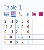
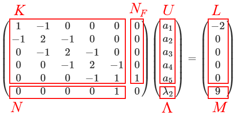
Recall our simple example of 1D heat transfer at steady state with no heat source, where the temperature T is a function of the position x in the domain defined by the interval 1 \le x \le 5. We imposed the Neumann boundary condition such that the outgoing flux should be 2 at the left boundary (x=1) and the Dirichlet boundary condition such that the temperature should be 9 at the right boundary (x=5). After discretizing the weak form equation, we obtained this matrix equation:
\begin{array}{cccccc}
1 & -1 & 0 & 0 & 0 & 0 \\
-1 & 2 & -1 & 0 & 0 & 0 \\
0 & -1 & 2 & -1 & 0 & 0 \\
0 & 0 & -1 & 2 & -1 & 0 \\
0 & 0 & 0 & -1 & 1 & 1 \\
0 & 0 & 0 & 0 & 1 & 0
\end{array}
\right)
\left(
\begin{array}{c} a_1 \\ a_2 \\ a_3 \\ a_4 \\ a_5 \\ \lambda_2 \end{array}
\right)
= \left(
\begin{array}{c} -2 \\ 0 \\ 0 \\ 0 \\ 0 \\ 9 \end{array}
\right)
where a_1, a_2, \cdots , a_5 are unknown temperature values at the nodal points (x=1, 2, \cdots, 5) and \lambda_2 is an unknown heat flux at the right boundary (x=5). The matrix on the left-hand side is customarily called the stiffness matrix and the vector on the right is called the load vector, due to the application of this technique in structural mechanics.
Viewing the Stiffness Matrix and Load Vector
The steps for implementing the weak form equation in COMSOL Multiphysics have been discussed in this earlier blog entry, thus we will not repeat them here. To view the stiffness matrix and load vector, right-click Solution 1 in the model tree → Other → Assemble, as shown in the screenshot below:
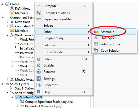
Make sure to drag the Assemble node up to position it above (before) the Stationary Solver node. If this step is not done and the Assemble node is left below (after) the Stationary Solver node, then the content of the load vector may be altered by the solver.
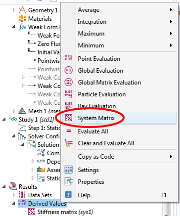
Then, in the settings window for the Assemble 1 node, we can select the matrices of interest by checking the corresponding checkbox for each item. Additionally, set Scaling of Dependent Variables 1 to None. After solving, we can evaluate the matrices by right-clicking Derived Values and then selecting System Matrix, as illustrated below:
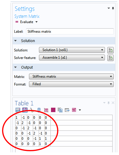
In the corresponding settings window, we can select Stiffness matrix from the Matrix drop-down menu and evaluate it in a table. As indicated in the screenshot below, we obtain exactly the same 6×6 matrix as the one in Eq. (1).
The load vector on the right-hand side of Eq. (1) can be evaluated and verified by the same procedure.
Pointwise Constraint
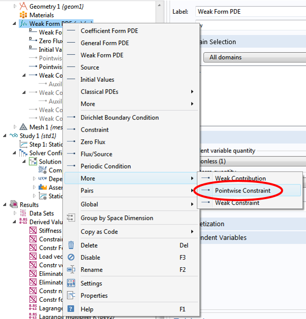
We mentioned before that it is sometimes desirable not to solve for the Lagrange multiplier \lambda_2 — for example, to save computation resources. To do so, we right-click the Weak Form PDE main node → More → Pointwise Constraint, as depicted below:
Then, in the settings window, we enter 9-T for the Constraint expression input field. After solving, we obtain exactly the same solution, but a smaller 5×5 stiffness matrix:
If we look at this matrix closely, we find that it matches the upper left-hand part of the 6×6 matrix that we observed earlier. This should not be too surprising, as we are solving exactly the same problem (represented by Eq. (1)), just in a slightly different way. We will briefly discuss this next.
Alternative Methods for Solving the Matrix Equation
When we implement the Dirichlet boundary condition using the Weak Contribution feature with a Lagrange multiplier \lambda_2 (as shown in this previous blog post), we effectively ask that the entire matrix equation (1) be solved to yield the coefficients a_1, a_2, \cdots , a_5 as well as the multiplier \lambda_2.
On the other hand, when we implement the fixed boundary condition using the Pointwise Constraint feature as shown above, we essentially ask that the same matrix equation (1) be solved without explicitly solving for the Lagrange multiplier \lambda_2. The software effectively segregates Eq. (1) to this form (see below)
K & N_F \\
N & 0 \end{array}\right)
\left(\begin{array}{c}
U \\
\Lambda \end{array}\right)
=
\left(\begin{array}{c}
L \\
M \end{array}\right)
where the stiffness matrix K is the 5×5 matrix shown above, the constraint Jacobian matrix N is (0 \, 0 \, 0 \, 0 \, 1), the constraint force Jacobian matrix N_F is (0 \, 0 \, 0 \, 0 \, 1)^T, the solution vector U is formed by the coefficients a_1, a_2, \cdots , a_5, the (one-element) vector \Lambda is formed by the Lagrange multiplier \lambda_2, the load vector L is (-2 \, 0 \, 0\, 0\, 0)^T, and the (one-element) constraint vector M is (9).
This segregation of Eq. (1) is shown graphically below:
Of course, in reality, when the Pointwise Constraint feature is specified, the software does not bother to assemble the full 6×6 matrix in Eq. (1). Instead, it assembles K, N, and N_F, which requires less computational resources than assembling the full matrix.
Eq. (2) can be written as a system of two matrix equations:
where the first one (3) contains the part of the discretized weak form equation with heat flux boundary conditions and the second one (4) contains the constraint imposed by the Dirichlet boundary condition.
The equation system can be solved in two steps. In the first step, the constraint equation (4) is solved for the degree(s) of freedom involved with the Dirichlet boundary condition. In the second step, the solution from the first step is substituted into Eq. (3) to solve for the remaining degrees of freedom.
The resulting solution vector U is then given as the linear combination of the solutions from the two steps:
(5)
The first term U_d is the solution vector of the constraint equation (4) solved in the first step. The second term is obtained from the second step in the form of the product of a matrix Null and a solution vector U_n. The columns of the matrix Null are formed by the basis vectors spanning the null space of the constraint Jacobian matrix N. So, we have
The solution vector U_n is the solution to the eliminated matrix equation
where the eliminated stiffness matrix K_c and the eliminated load vector L_c are given by
K_c& = Nullf^T \, K \, Null \\
L_c& = Nullf^T \, (L-K \, U_d)
\end{align}
and the columns of the matrix Nullf are formed by the basis vectors spanning the null space of the transpose of the constraint force Jacobian matrix N_F. So, we have
The term eliminated indicates that the degree(s) of freedom involved in the Dirichlet boundary condition have been removed from the matrix equation (6). In our example, the size of the eliminated stiffness matrix K_c is 4×4.
Notice that the solution procedure described above does not involve the Lagrange multiplier vector \Lambda. Indeed, the value of the Lagrange multiplier \lambda_2 is left unsolved by this procedure. The advantage of this method is that the required computational resources are reduced. For our simple example, the size of the matrix is reduced from 6×6 to 4×4 (plus an even smaller one for the constraint equation).
Viewing All Matrices at Once with a COMSOL® App
COMSOL Multiphysics allows us to evaluate and view any of the matrices and vectors mentioned above. All we have to do is to follow the same procedure outlined in the previous section on viewing the stiffness matrix and load vector. However, we quickly find out that we will spend a lot of time clicking on each System Matrix node in the Model Builder and then clicking on the “Evaluate” button in the settings window. Also, we can only see one matrix or vector at a time, making it tedious to examine all the matrices and vectors.
This represents one of the many situations in which a COMSOL application can help enhance modeling experience and productivity (learn about application webinars below). The core package of COMSOL Multiphysics can be used to build a COMSOL app based on any COMSOL model by wrapping a user interface (UI) around it. The UI is completely customizable and can be easily configured to suit individual modeling needs.
For an introduction to COMSOL applications, see the following webinars: Intro to COMSOL Multiphysics® 5.0 and the Application Builder (with a focus on the second half) and How to Build and Run Simulation Apps with COMSOL Server™.
The following screenshots show just one of the essentially infinite number of ways that a UI can be arranged to serve as a convenient tool for investigating the matrices and vectors. The app is set up to switch among several different kinds of boundary conditions via checkboxes. All matrices and vectors are evaluated and displayed by a single click of the “Compute” button. Here is a screenshot of the case in which the full 6×6 matrix is used to solve:
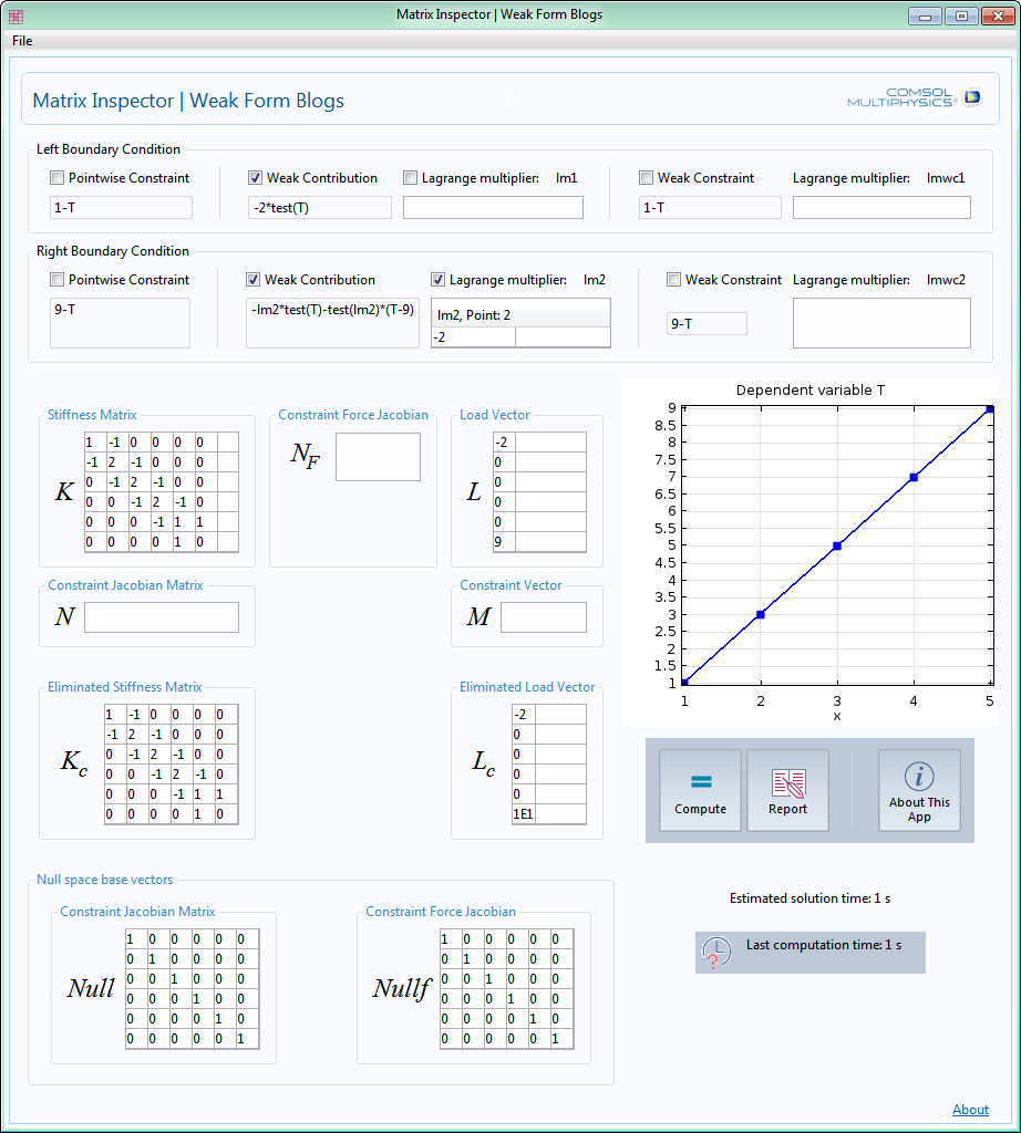
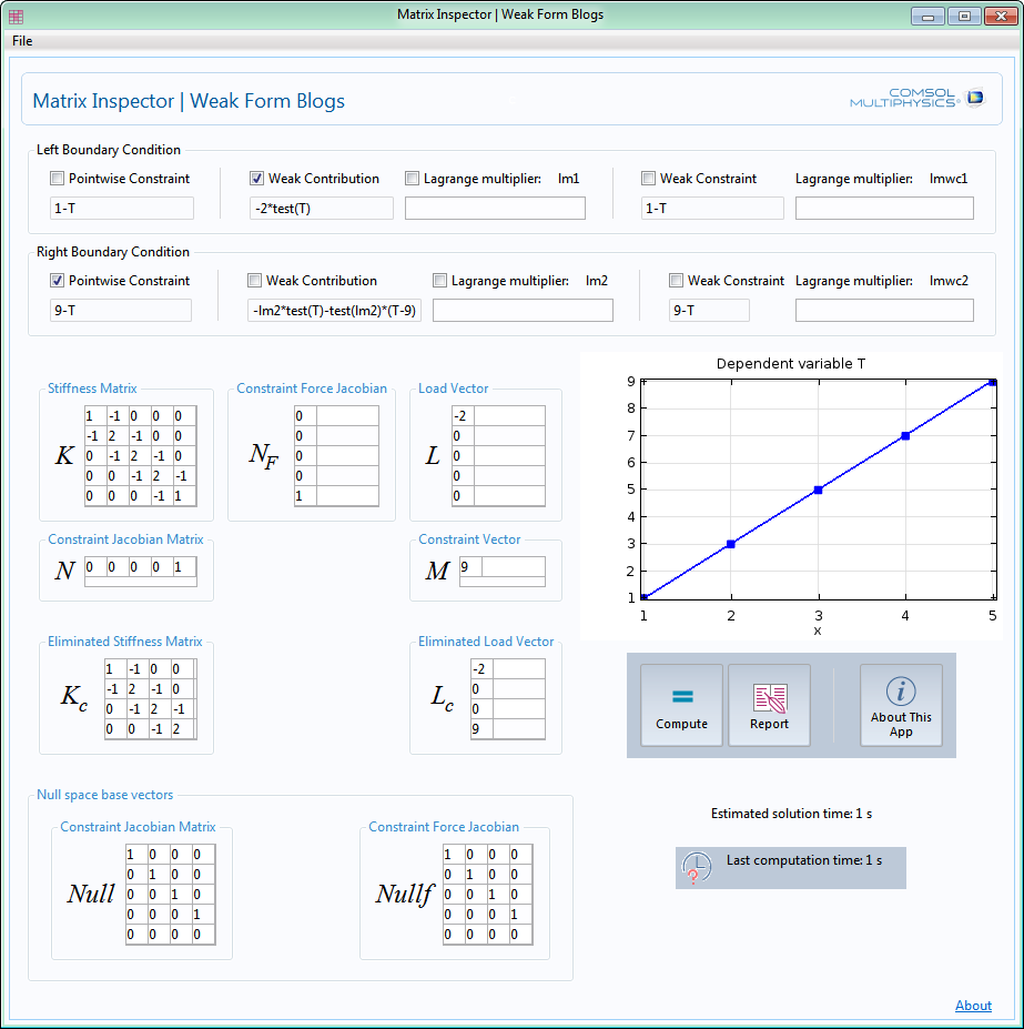
We see that N, N_F, and M are empty and K_c remains the full size of 6×6. In contrast, here is the screenshot for the second case where the eliminated 4×4 matrix is used to solve:
Concluding Remarks
Using our simple heat transfer example, we have explored the two different ways to solve the matrix equation obtained from discretizing the weak form equation. We found that it can be much simpler to evaluate and inspect the various matrices and vectors involved in the solution process by setting up a COMSOL application. In the next blog posts, we will continue to use COMSOL apps to help us investigate more complex examples.
As a general-purpose development environment for multiphysics simulation, the COMSOL Desktop® environment must be structured with a limited arrangement of UI elements. The COMSOL app frees us from such limitations, providing the power for building specialized UI for unique requirements. Additionally, the built-in coding functionality allows much more versatile computations, and COMSOL Server™ license enables the deployment of apps for worldwide access by coworkers as well as clients.
We hope that you will use these powerful features in COMSOL Multiphysics to boost your own work efficiency!


Comments (18)
Tae Eun Kim
June 16, 2015Can I get this app if it is possible? thanks.
Jing Wang
July 6, 2015Dear Chien,
I‘ve followed your instruction step by step in my comsol 5.0, however, i couldn’t get the same load vector as yours although i got the same stiffness matrix. My load vector is
0
0
-8.881784197001252E-16
1.7763568394002505E-15
-1.1102230246251565E-15
0
instead of
-2
0
0
0
0
9
Can you please post your mph.file here so i can check it out?
Thank you anyway!
Best regards,
Jing
Chien Liu
July 13, 2015 COMSOL EmployeeDear Jing,
Thank you for the comments. Most likely the boundary conditions were not specified as described. If you need further assistance, please contact us at
support@comosl.com
Sincerely,
Chien
Jing Wang
July 15, 2015Jing Wang
July 18, 2015Dear Chien,
Thanks for your reply! I’ve checked the boundary conditions, they are just the same as those in your post “Implementing the Weak Form in COMSOL Multiphysics”. Can you please send your mph.file to me (My email: comsol@foxmail.com)? Thank you anyway!
Sincerely,
Jing
Chien Liu
July 20, 2015 COMSOL EmployeeDear Jing,
Thank you for following up and please contact us at
support@comsol.com
Sincerely,
Chien
Roland Ernst
February 9, 2016Dear Chien,
Very interesting blog about how the weak_form is implemented in Comsol! I followed a specialized Comsol seminary about these aspects about 10 years ago and would like to remind this again. So I have 2 questions about that:
1/ I have not understood how the matrices Null, Kc and Lc are formed. What means for example your sentence: “Null are formed by the basis vectors spanning the null space of the constraint Jacobian matrix N”? Is there a book or some publications about all these aspects and more specifically the theory of Lagrange multipliers?
2/ I have not completely understood what is the difference between ideal and non ideal constraints and when to use either one or the other one (I think now this has been replaced by options like “apply reaction terms on all physics/or individual dependant variables”). Could you please give me some explanations about that and how it influences the former matrices and also what’s the physical signification of this? A blog about that special aspect would also be very appreciated!
Thanks in advance for your help!
Sincerely
Roland
Chien Liu
February 9, 2016 COMSOL EmployeeDear Roland,
Thank you for the comments!
Regarding the questions, you should be able to find more information in the COMSOL Multiphysics Reference Manual > Equation-Based Modeling > Modeling with PDEs > About Weak Form PDE (and the following sections). And yes we plan to continue the blog series with more topics on the constraints. Thank you for your interest in this.
Sincerely,
Chien
Roland Ernst
February 16, 2016Dear Chien,
Thank you for your comments. But sorry when I go to your mentioned Comsol documentation I find nothing speaking about the Null, Kc, Lc (etc…) matrices you use in your weak form implementation explanations of your blog. Could you please give me some more details about for instance your Null matrix is built? Meaning I don’t understand what you mean by saying ” The columns of the matrix Null are formed by the basis vectors spanning the null space of the constraint Jacobian matrix N” . Thank you for your help!
Regards
Roland
Evgeni Sergeev
March 10, 2016Thank you very much for the blog series. A tremendous value-adder to Comsol. I think this is helping every user of Comsol who is serious about understanding what they’re doing, and not just generating pretty pictures.
If anybody is interested in condition numbers, just wanted to add that computing cond(K) is meaningless, while cond(Kc) is correct. (Even though K is called the “stiffness matrix”, so that one might intuitively attempt to compute its condition number.) It’s the equation Kc×Un=Lc that gets sent to the linear solver, so Kc is the relevant one. The condition number of the original system
cond([ms.K ms.NF; ms.N zeros(size(ms.N,1))])
might also make sense to check [in my case this is similar to cond(Kc)], but not cond(K).
I suspect that the condition number is somehow related to LinErr (trying to understand why the relative error in my model is so high, when the residual is plotted as zero everywhere and LinRes is ~1e-15). This isn’t clear from how LinErr is defined in the documentation, but they seem correlated to some extent.
wang shuo
March 13, 2016I think there might be a error about the load vector which should be,
(-2,0,0,0,0,\lamda_2)^T
and also the solution vector,
(a_1,a_2,a_3,a_4,a_5,9)^T
Please correct me if I am wrong
Chien Liu
March 15, 2016 COMSOL EmployeeDear shuo,
\lambda_2 belongs to the vector formed by U and \Lambda. Please see Eq. (2) and the graph below it.
Sincerely,
Chien
Evgeni Sergeev
June 20, 2016I’ve ran into the same issue as Jing Wang above: the load vector entries are all zero or near machine epsilon.
I posted my 1-element MPH model and a detailed description on the forum:
https://www.comsol.com/community/forums/general/thread/116751/#p259471
It also shows a way to get the load vector, by messing with “Linear perturbation” settings. I don’t fully understand the meaning of that, but it may be of interest for those who wish to get the matrices using LiveLink and solve in Matlab.
Regards,
Evgeni
Chien Liu
June 20, 2016 COMSOL EmployeeDear Evgeni,
Thank you for the comment. Did you perform this step as described in the text of the blog post: “Make sure to drag the Assemble node up to position it before the Stationary Solver node.” ?
If this step is not done and the Assemble node is left after (below) the Stationary Solver node, then the content of the load vector may be altered by the solver as you have observed.
Hope this helps.
Sincerely,
Chien
ChienShun Liu
July 31, 2020Dear Chien:
I saw in your post ‘Implementing the Weak Form with a COMSOL App’
how to extract/view the stiffness matrix and the right hand side Lc.
I wonder if it is possible to extract the (extended) mass matrix without
using Livelink?
Problem description:
Lap u = f in Omega
u = g_D on Gamma_1 (pointwise constraint)
du/dn = g_N on Gamma_2 (natural BC)
By extended mass matrix I mean one that takes
the input (f_DOF,g_D,g_N) and out put to the
right hand side Lc in the final equation
Kc u = Lc
Here f_DOF means the point values of the source term f
on the degrees of freedom (nodes) of the underlying finite element
method.
Chien Liu
July 31, 2020 COMSOL EmployeeDear ChienShun, If you meant Eq. (6) then yes, as you can see in the last screenshot in the post, Kc and Lc are evaluated. No LiveLink products are used in the App, only the base package is used. If you need further assistance, please contact us using your COMSOL support portal (log in to your COMSOL Access account at https://www.comsol.com/access and then click on the Submit New Support Case button). Sincerely, Chien
Nmisha Arora
March 26, 2021Sir, I have implemented this model in COMSOL 5.5, as described in this blog post and earlier posts. I didn’t get the exact same stiffness matrix but the load matrix was up-to mark.
Following is what I get:
2.3333 -2.6667 0.33333 0.0000 0.0000 0.0000 0.0000 0.0000 0.0000 0.0000
-2.6667 5.3333 -2.6667 0.0000 0.0000 0.0000 0.0000 0.0000 0.0000 0.0000
0.33333 -2.6667 4.6667 -2.6667 0.33333 0.0000 0.0000 0.0000 0.0000 0.0000
0.0000 0.0000 -2.6667 5.3333 -2.6667 0.0000 0.0000 0.0000 0.0000 0.0000
0.0000 0.0000 0.33333 -2.6667 4.6667 -2.6667 0.33333 0.0000 0.0000 0.0000
0.0000 0.0000 0.0000 0.0000 -2.6667 5.3333 -2.6667 0.0000 0.0000 0.0000
0.0000 0.0000 0.0000 0.0000 0.33333 -2.6667 4.6667 -2.6667 0.33333 0.0000
0.0000 0.0000 0.0000 0.0000 0.0000 0.0000 -2.6667 5.3333 -2.6667 0.0000
0.0000 0.0000 0.0000 0.0000 0.0000 0.0000 0.33333 -2.6667 2.3333 1.0000
0.0000 0.0000 0.0000 0.0000 0.0000 0.0000 0.0000 0.0000 1.0000 0.0000
Chien Liu
March 26, 2021 COMSOL EmployeeDear Nmisha, Looks like you did not follow the previous post
https://www.comsol.com/blogs/implementing-the-weak-form-in-comsol-multiphysics/
which selects the Linear element order. Sincerely, Chien