

The release of COMSOL Multiphysics version 5.0 includes a new add-on module for electromagnetics modeling: the Ray Optics Module. This optional add-on module includes the Geometrical Optics interface, which can be used to model the propagation of electromagnetic waves when the wavelength is much smaller than the smallest geometric entity in the model. The Geometrical Optics interface includes a wide variety of features and optional settings and it is fully multiphysics capable.
Geometrical Optics, Beam Envelopes, or Full-Wave Electromagnetics?
COMSOL Multiphysics has three add-on products for electromagnetic wave propagation: the Ray Optics Module, the Wave Optics Module, and the RF Module. Let’s take a look at the differences.
Full-Wave Electromagnetics
The RF Module and the Wave Optics Module both offer an Electromagnetic Waves, Frequency Domain interface, which solves the full-wave form of Maxwell’s equations via the finite element method (FEM). This requires a finite element mesh that is fine enough to resolve the electromagnetic waves, as shown in the figure below.
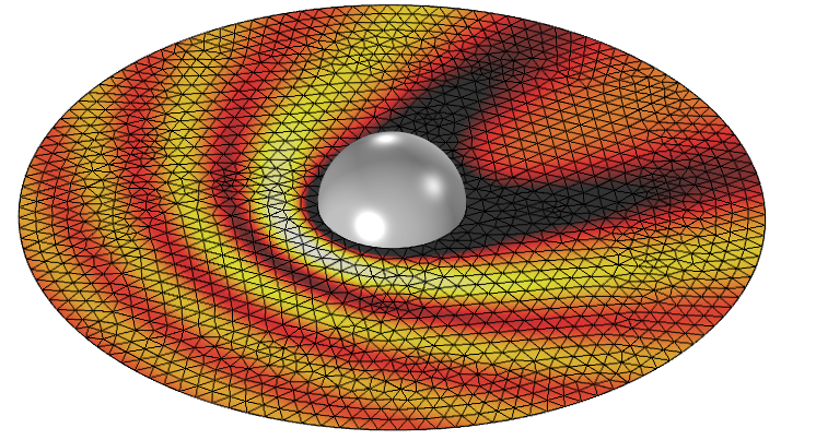
Full-wave simulation of scattering off of a metallic sphere. The variations in the magnitude of the electric field require a fine mesh everywhere.
This approach is appropriate when the solutions we are interested in have significant variations in all directions and are on a length scale comparable to the wavelength.
Beam Envelopes
The Wave Optics Module also includes the Electromagnetic Waves, Beam Envelopes interface, which solves a modified version of the full-wave Maxwell’s equations, again via the finite element method. The Beam Envelopes formulation requires, as input, an approximate and slowly varying wave vector. Rather than solving for the electromagnetic fields themselves, this formulation solves for the slowly varying electric field amplitude.
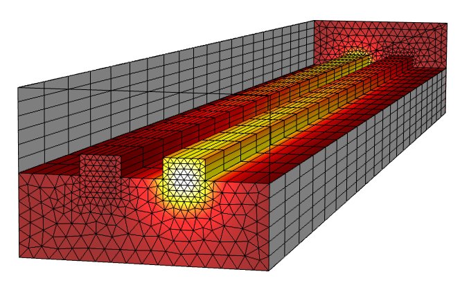
Beam envelopes simulation of a directional coupler. The gradual variation in the field magnitude allows for a very coarse mesh in that direction.
The advantage of the Beam Envelopes formulation is that a very coarse mesh can be used in the direction of propagation. The limitation is that the wave vector field must be approximately uniform or slowly varying throughout the modeling domain. However, this is indeed the case for a range of important optical devices such as optical fibers or directional couplers.
Geometrical Optics
The Ray Optics Module includes the Geometrical Optics interface, which treats electromagnetic waves as rays. It does not use the finite element method; instead, it traces the rays through the modeling domain by solving a set of ordinary differential equations for the position and wave vector. Although the domains through which the rays travel must be meshed, the mesh can be very coarse. Only at curved surfaces must the mesh be refined.
Editor’s note: As of COMSOL Multiphysics® version 5.2a, the surrounding empty space around an optical system no longer needs to be meshed. For more details, see the Release Highlights page.
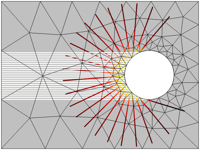
Geometrical optics simulation of a plane wave scattering from a cylinder. The ray intensity decreases after the rays are reflected by the curved surface, causing the waves to diverge. A very coarse mesh can be used, except on the curved boundaries.
What’s in the Ray Optics Module?
The Ray Optics Module traces rays of light propagating through different media and can consider many different behaviors of the rays at boundaries. The wavelength-dependence of the refractive indices of the media can be considered. It is also possible to compute the intensity, the phase, and the polarization of light and how these vary as the ray goes through different media and across boundaries.
Let’s now take a deeper look at the various physical phenomena that can be modeled.
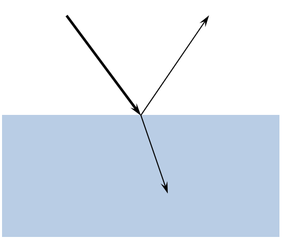
Refraction and reflection at a dielectric interface.
A ray of light propagating through a medium of uniform refractive index will travel in a straight line. When the ray encounters an interface between materials of different refractive indices, the ray will be partially reflected and partially refracted. This behavior is governed by Snell’s Law and the Fresnel equations and is handled automatically, by the Ray Optics Module, at interfaces between different materials.
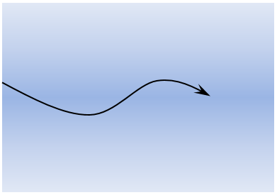
A light ray bends as it passes through a graded index material.
Light propagating through a medium with a non-uniform refractive index will bend in the direction of a relatively higher refractive index. Such graded index behavior can be modeled simply by defining the refractive index as a smooth, spatially varying function. The Ray Optics Module inherits the powerful tools of COMSOL Multiphysics for creating spatially varying materials.
For instance, the Luneburg Lens example model available in the Model Library of the Ray Optics Module defines the refractive index simply as sqrt(x^2+y^2+z^2). Alternatively, you can define spatially distributed media as a look-up table from a file, or more spectacularly, as a function of another physics field quantity such as n = f(T(x,y,z)), where n is the refractive index, f is some function, and T(x,y,z) is a spatially varying temperature field computed by a heat transfer simulation in COMSOL Multiphysics. More on this in a blog post coming soon.
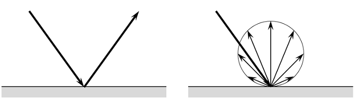
Specular (left) and diffuse (right) reflection of a ray of light.
At boundaries, the ray can propagate through unimpeded as if the boundary were completely transparent, it can be completely absorbed, or it can be reflected. Reflections occur at surfaces of materials through which light cannot pass and will be either specular, diffuse, or a mixture of the two. Specular reflection occurs on highly polished metal surfaces, whereas most other surfaces reflect more diffusely.
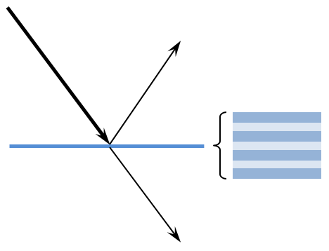
Reflection and transmission through a (possibly multi-layer) thin dielectric film.
It is also possible to model structures composed of thin layers of different materials, such as dielectric mirrors or antireflective coatings. These can be modeled by adding one or more Thin Dielectric Film nodes to a boundary. The effective reflection and transmission coefficients through the multi-layer stack are then computed without explicitly modeling each layer. This is demonstrated in the Antireflective Coating, Multilayer model.
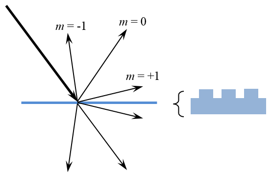
Reflection and transmission into various diffraction orders from an optical grating.
On the other hand, structures with periodic wavelength-scale variation in the plane of the boundary can be modeled with the Grating boundary condition. Diffraction gratings have periodic variations in their structure and can split and diffract a ray into several different rays, which are termed diffraction orders. It is also possible to compute the characteristics of the grating via the full-wave formulation and use this as an input, as demonstrated in the Diffraction Grating model.
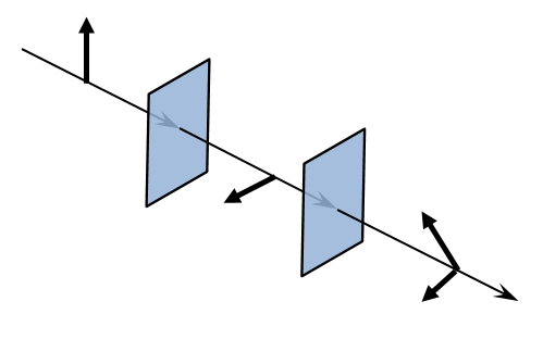
The polarization of a ray of light changes as it goes through various optical elements.
Lastly, boundary conditions can be used to manipulate the polarization of the ray. Boundary conditions for simulating linear polarizers, linear and circular wave retarders, ideal depolarizers, and optical components with arbitrary Mueller matrices can be represented as boundary conditions. These conditions are demonstrated in the Linear Wave Retarder model.
The rays themselves can be launched into the model from domains, boundaries, and any user-specified points. The rays can have a spherical, hemispherical, or conical distribution. It is also possible to model illumination from the Sun by specifying a position on Earth. Along with the path of the ray, the intensity, polarization, and phase can also be computed, if desired. This makes it possible to compute both optical intensity on surfaces and interference patterns. Examples of this include modeling a solar dish and computing the interference pattern of a Michelson interferometer.
What’s Not in the Ray Optics Module?
The Ray Optics Module does not directly consider interactions with structures that have size comparable to the wavelength.
For example, consider a plane wave scattering off of a diamond-shaped metallic object as shown below. If the wavelength is comparable to the object size, there will be significant diffraction around the object and the region behind it will get illuminated. Similarly, a plane wave incident upon a wavelength-scale slit will experience significant diffraction and broadening. Modeling either of these effects requires a full-wave approach using the Wave Optics Module or the RF Module.
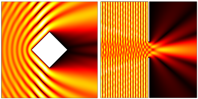
A diamond-shaped object scatters an electromagnetic wave in all directions (left). There is significant illumination behind the scatterer. A plane wave incident upon a slit (right) will spread out. The color in both plots indicates the electric field norm.
The Geometrical Optics approach, on the other hand, does not consider these diffractive phenomena. Rays representing a plane wave will be reflected specularly from the surfaces and will not illuminate the region behind the object. Rays passing through a slit will not spread out. These are both valid approximations if the wavelength of light is much smaller than the object’s size.
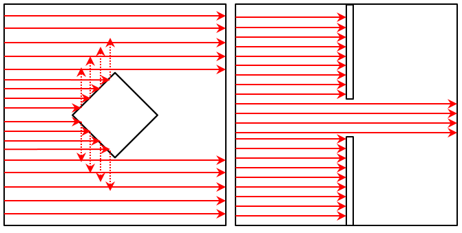
A diamond-shaped object in a plane wave using the Geometrical Optics approach (left) and a plane wave passing through a slit (right) does not experience any diffraction.
Currently, the Ray Optics Module also does not consider refractive indices that are dependent upon the intensity of light. However, such problems can be addressed with the Beam Envelopes formulation in the Wave Optics Module, as demonstrated in the example of Self Focusing in BK-7 Glass.
Summary and Next Steps
The complete capabilities of the Ray Optics Module are demonstrated by the Model Library examples, available within the software and on our online Model Gallery.
If you are interested in using the Ray Optics Module for any of your modeling needs, please contact us.

Comments (3)
RAFAEL SARAIVA CAMPOS
March 22, 2016Walter,
First of all, thanks and congratulations for all your excellent posts.
Second, would you happen to have the COMSOl file used to generate the figure displaying the diamond-shaped object scattering an electromagnetic wave, shown in this post?
I am using the RF Module to simulate RF propagation within a 2D geometry representing the blueprint of a building floor, and I need to taken diffraction into consideration in my model, but, as I am new to COMSOL, I haven’t been able to do so yet.
Thank you in advance,
Your sincerely,
Rafael Saraiva campos
Surendra Singh
October 28, 2022Dear Walter,
I am new to COMSOL and learning to use Ray Optics module. I plan to use it for raytracing in a medium which is defined by numerical data – refractive index n(x,y,z) as a function of f(D(x,y,x)) density field around an object moving in a fluid. I hope your new blog will address how to construct a geometry inside Ray Optics module using this data in a file. If there is something that already exists addressing a similar problem, I would like to know. Thank you.
SPS
Walter Frei
October 28, 2022 COMSOL EmployeeHello Surendra,
This is an interesting question, but a bit outside of a blog topic. We would suggest that you contact the COMSOL Support Team for personalized assistance with this.