
Performing uncertainty quantification (UQ) studies can help engineers understand how uncertainties affect model predictions and design performance. When experimental data is available, inverse uncertainty quantification (IUQ) can be used to calibrate model parameters while accounting for uncertainty. In this blog post, we demonstrate how to perform an IUQ study in the COMSOL Multiphysics® software and how to use the resulting posterior distributions in a forward UQ study.
Defining IUQ
In our previous blog post “How Reliable Is Your Resistor?”, we discussed how forward UQ predicts how variations in material properties, geometry, or manufacturing processes affect a resistor’s performance. In many cases, however, measurement data is already available (e.g., resistance values from experiments), and it becomes more interesting to calibrate the input parameters, especially the material properties. In the COMSOL® software, IUQ can be used for this task, as it works backward from observed data to estimate those unknown inputs, combining the finite element method with surrogate models to efficiently calibrate the input parameters.
While parameter estimation focuses on identifying the best fit parameter values, IUQ provides a probabilistic description of the calibration parameters, including their likely ranges, confidence levels, and correlations. By refining parameter distributions based on measurements, IUQ improves model accuracy and predictive capability.
Moreover, it’s often desirable to perform an IUQ study when experimental data is available and input distribution is unknown. For example, after identifying key parameters using screening or a sensitivity analysis, an IUQ study can be used to obtain posterior distributions for these parameters. These calibrated distributions can then be used as input parameters for a forward UQ study like uncertainty propagation and reliability analysis. This procedure creates a more realistic workflow since the uncertainties used for prediction are informed by data and the prior assumption.
Here, we will discuss how to perform an IUQ study and how to seamlessly use the resulting posterior distributions in a forward uncertainty propagation study in the COMSOL® software.
Understanding IUQ with a Resistor Model
IUQ estimates calibration parameters by combining experimental data with prior knowledge. It can be viewed as parameter estimation in a Bayesian framework, where measurements guide the updating of parameter distributions.
The experimental data provides the reference quantities that the model must reproduce, such as the measured resistance at different applied voltages in a resistor. During an IUQ study, COMSOL® evaluates how likely it is for each parameter set to occur by comparing simulated outputs with these measurements.
In the software, IUQ compares the experimental data with predictions from a surrogate model trained using finite element simulations. The finite element model defines the physics-based relationship between uncertain inputs and measurable outputs, whereas the surrogate model approximates this relationship and enables efficient sampling of the parameter space.
The Bayesian updating process combines prior distributions with a likelihood function that measures the consistency between surrogate predictions and experimental data. The resulting posterior distributions represent the most likely values of the calibration parameters together with their uncertainty. Through this process, IUQ provides calibrated material properties in a data-informed and computationally efficient way. Thus, experimental data directly influences the inferred parameter distributions.
Workflow: Performing IUQ in COMSOL®
Define the Problem and Build the FEM Model and IUQ Study
The first step of setting up an IUQ study is to create a physics-based model representing the system at hand. In the resistor example highlighted in our previous blog post, the Electric Currents interface is used to compute the resistance based on specified material properties and geometry. Two conductivities, Sigma1 and Sigma2, defined on different regions of the resistor, are selected as the calibration parameters. A stationary study establishes the forward relationship between the input parameters and the output quantity, which is the resistance. For our IUQ example, we will keep these settings.
The next step is to add an Uncertainty Quantification study, using Study 1 as the reference, and selecting Inverse uncertainty quantification as the study type. Both Gaussian process and polynomial chaos expansion approaches can be used as surrogate models for IUQ. In this example, an adaptive sparse polynomial chaos expansion is used. The variable comp1.Res, which evaluates the resistance of the resistor, is defined as the quantity of interest (QoI) and refers to the simulation output.
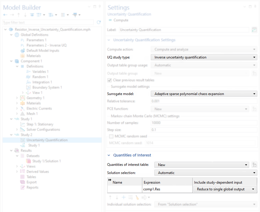 Figure 1. The Uncertainty Quantification study settings, with Inverse uncertainty quantification selected.
Define Uncertainty Input Parameters and Their Prior Distributions
Under Input Parameters, include both the calibration parameters (Sigma1 and Sigma2) and the experimental parameter, which is the applied voltage, V0. Each value of V0 corresponds to a different experiment. Therefore, V0 is treated as an experimental parameter rather than a calibration parameter.
Next, provide a prior distribution for each parameter. In this demonstration, normal distributions are assumed for Sigma1 and Sigma2. For the experimental parameter V0, a uniform distribution is used because the measurements are performed over a range of voltages.
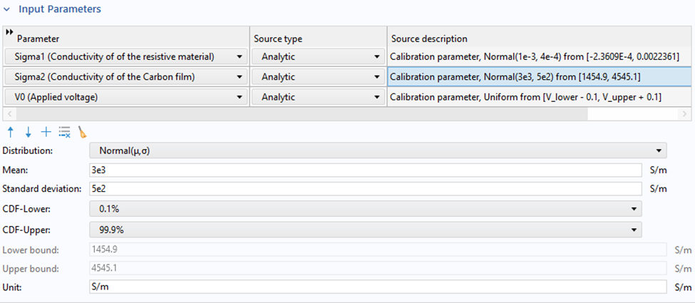 Figure 2. Input parameters and prior distributions.
The experimental parameter V0 must be included because the surrogate model represents the system response as a function of both the calibration parameters and the experimental condition. The bounds of the V0 distribution (e.g., from 4.9 to 35.1 V) should cover the voltage range used in the experiments, for example, from 5 to 35 V.
Prepare and Import Experimental Data
In the Experimental Data Settings section, experimental values can be provided in table format. External measurement data can be imported from files such as .txt or .csv. For this demonstration, pseudoexperimental resistance data is generated by running the Stationary study with an auxiliary sweep over the voltage V0. A measured resistance variable is defined as
where Res is the resistance evaluated from the finite element method (FEM) model and rn1() is a random function. The random function rn1() adds measurement noise to the simulated resistance. The evaluated values of Res_measured as a function of V0 are then selected in the Experimental data table in the IUQ settings.
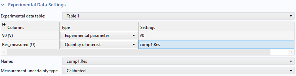 Figure 3. The experimental data settings with Calibrated selected as the measurement uncertainty type.
Here, V0 (the voltage parameter) is selected as the experiment parameter, and the pseudoexperimental data, Res_measured evaluated under Global Evaluation, is defined as the QoI.
If Measurement uncertainty type is set to Calibrated, COMSOL® estimates the measurement uncertainty as part of the IUQ process. If Experimental data is selected instead, the measurement uncertainty must be provided explicitly.
Samplings and Surrogate Model Settings
Under the sampling settings, the maximum number of input points can be specified, which directly controls the size of the training dataset generated from FEM simulations. These input points are used to train the surrogate model based on FEM simulations.
Note: In this demo model, before running the IUQ study, the Auxiliary sweep in the Stationary step should be disabled.
IUQ Results
The IUQ study produces the joint probability distribution and the calibrated confidence intervals shown in Figures 4 and 5, respectively. Figure 6 compares the prior and posterior distributions for Sigma1 and Sigma2, demonstrating how the experimental data refines the parameter estimates and reduces uncertainty, especially for Sigma2. Note that Sigma1 is the conductivity of the resistive material, and the resistance is insensitive to Sigma1, as demonstrated in the previous screening analysis. Thus, the prior and posterior distributions for Sigma1 are quite similar.
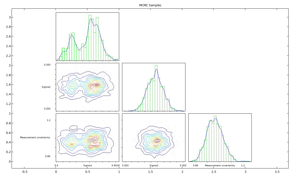 Figure 4. Joint probability distribution for Markov chain Monte Carlo (MCMC) samples.
 Figure 5. The calibrated confidence interval.
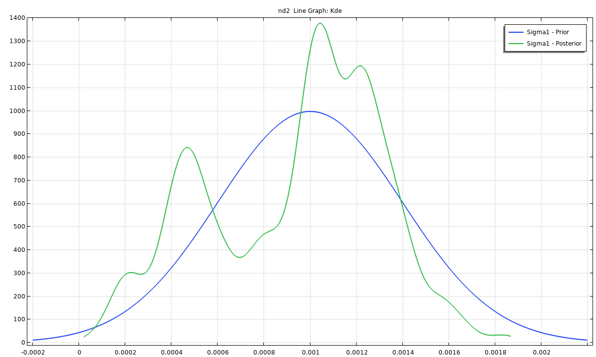
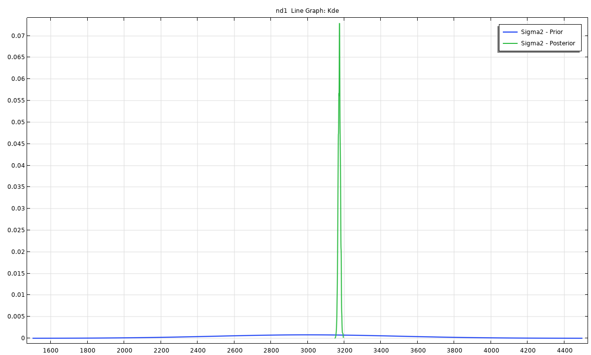
Figure 6. A comparison between the prior and posterior distributions for Sigma1 and Sigma2.
Using Posterior Distributions for a Forward UQ Study
The posterior distributions obtained from an IUQ study can be directly reused in a forward UQ study. To implement the distributions, the first step is to add a new Uncertainty Quantification study of type Uncertainty Propagation from the IUQ study.
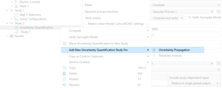 Figure 7. Adding a new UQ study for uncertainty propagation.
A new Quantities of Interest table is created automatically and is identical to the one used for the IUQ study. Since the same QoI, comp1.Res, is evaluated, either Analyze only or Improve and analyze can be selected. The former reuses the existing FEM data to train the new surrogate model, e.g., a new Gaussian Process model, while the latter allows additional simulations or input points to improve the surrogate model. For simplicity, we will use Analyze only for the forward UQ studies.
By default, a new Gaussian Process surrogate model is generated, which is used as the surrogate model for this new forward UQ study. From there, enable the new Gaussian Process and click Train Model. Through these steps, we can add the posterior distributions from the MCMC samples for the forward UQ study.
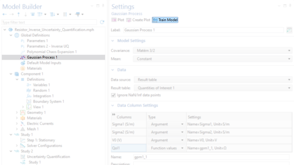 Figure 8. The settings for the Gaussian Process surrogate model.
Note that the distributions defined under the Input parameters section can be ignored for this forward UQ study. Instead, the posterior distributions obtained from the IUQ study fully define the sampling space. Therefore, no additional prior assumptions are required for the forward UQ sampling.
In the Surrogate-Based Monte Carlo Analysis section, select Manual for the Monte Carlo parameters source. Then, for each calibrated parameter, Sigma1 and Sigma2, select Data as the source type, Result table as the data source, and the corresponding column from the MCMC samples table for each parameter.
Note that we can select only one working condition for V0, which is the nominal value of 1 V.
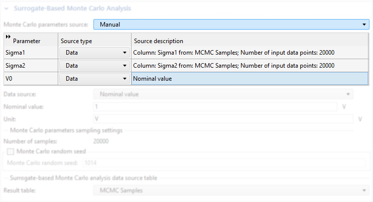 Figure 9. The settings in the Surrogate-Based Monte Carlo Analysis section for using the posterior distributions.
After this forward UQ study is finished, the kernel density estimation (KDE) plot based on the posterior distributions can be generated. This KDE reflects the uncertainty propagated from the calibrated parameter distributions. Figure 10 shows that the highest probability density of the resistance is located around 50 \Omega. According to the QoI confidence interval table (not shown), the mean predicted resistance is 49.975 \Omega, with a standard deviation of 0.0957 \Omega.
Similarly, a reliability analysis can be performed with the posterior distributions specified in the Surrogate-Based Monte Carlo Analysis section (Figure 9). For example, the probability of the resistance that is larger than 50.25 \Omega and 52.5 \Omega is approximately 2.55 and 0%, respectively. This probability quantifies the risk of exceeding specified resistance thresholds. Another way to say this is that we know that this resistor is more reliable for any applications requiring a precise 50 \Omega load.
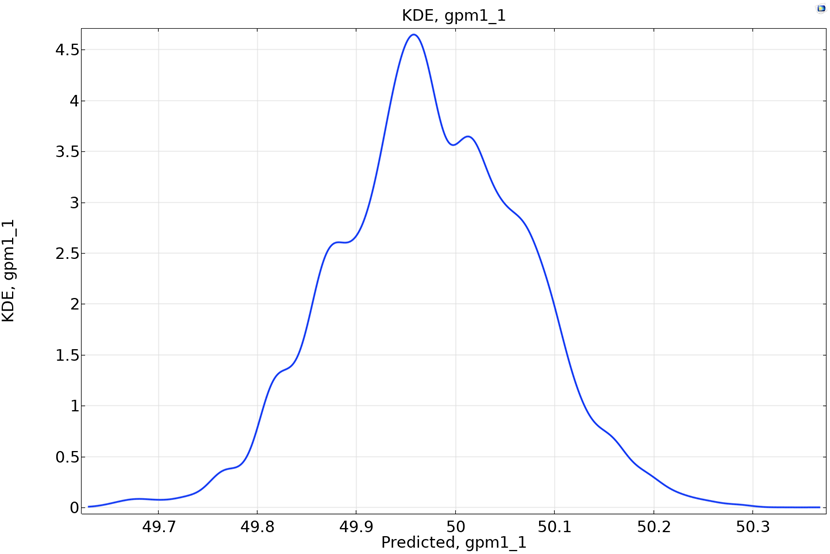 Figure 10. The KDE plot using posterior distributions.
A Data-Informed Workflow for Calibration and Uncertainty Propagation
Inverse uncertainty quantification provides a systematic way to calibrate uncertain input parameters using experimental data. By combining finite element modeling, surrogate modeling, and Bayesian updating, IUQ refines prior assumptions into posterior distributions that better represent the physical system.
When these posterior distributions are subsequently used in a forward UQ study, the predictions become more realistic and data informed. Instead of relying on assumed parameter variations, the uncertainty propagation is based on calibrated parameter distributions that reflect both measurements and model physics.
This combined workflow of IUQ followed by forward UQ enables more reliable prediction, improved confidence in simulation results, and a clearer understanding of how parameter uncertainty influences system performance. This workflow integrates model calibration and uncertainty propagation and can be completed within the COMSOL® software’s dedicated user interface, without needing to switch tools.
Next Steps
Want to learn more and try out the model discussed above? Download the related MPH file below:


Comments (0)