
Thermoacoustic engines generate acoustic energy from a thermal input. In contrast to commonly used engines such as reciprocating engines and gas turbines, thermoacoustic engines do not use moving parts, which keeps the structure very simple. In this blog post, we will see how the working mechanisms of thermoacoustic engines can be modeled with the Thermoviscous Acoustics interface, one of the powerful interfaces in the COMSOL Multiphysics® software for modeling the linearized behavior of a fluid.
How Thermoacoustic Engines Work
More than 150 years ago, Professor Pieter Rijke reported an interesting phenomenon that can be regarded as pioneering work on thermoacoustics. He put wire gauze in a glass cylinder tube, held vertically, and heated the gauze from the bottom using fire. After putting out the fire, he observed that the cylinder kept producing sound for a while. (Ref. 1) The apparatus is now well known as the Rijke tube, so some may have seen it used as an example of a resonant phenomenon. However, setting aside the resonance, how are the sounds generated in the first place?
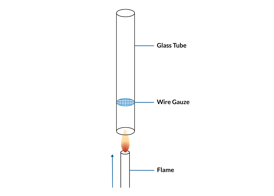
The Rijke tube setup.
The trick is the interaction between the temperature change and the fluid motion inside of the tube: The heated wire gauze induces natural convection of the air, making a steady flow through the pipe; thus the air above the wire gauze is warmer than the air below the wire gauze. At the standing half-wave acoustic resonance in the pipe, the air will flow through the wire gauze in both directions at different times in the acoustic period. As the air flows through the gauze, it will be heated. Since the air below the gauze is colder than the air above, more heat will be transferred when the flow is upward rather than downward. To obtain a sustained acoustic field, the heat release needs to be in phase with the pressure field, such that the fluid is heated when the acoustic pressure is positive. In a standing wave, the velocity field, which causes the heating, is out of phase with the pressure field. However, due to effects caused by the viscous boundary layers surrounding the wire gauze, the heat release is delayed compared to the velocity field. This phase delay causes the heat release to be partly in phase with the pressure field and results in a sustained resonance. If the pipe is turned sideways, the convection stops, and the resonance will no longer be sustained. If the pipe is turned upside down, the heat transferred will be largest when the acoustic pressure is negative, and therefore the acoustic field will be attenuated instead of sustained.
This is an example of the energy conversion between heat and acoustic energy. In fact, the whole apparatus demonstrates the working principles of thermoacoustic engines.
Thermoacoustic engines have a closed tube-like passage in which a sound can propagate, and a heat exchanger is in the passage to heat up or cool down the working fluid. Thermoacoustic engines use either standing waves or traveling waves, whereas the Rijke tube uses only standing waves. The traveling-wave engines are expected to realize better performance compared to standing waves due to the phase delay between the pressure and the fluid displacement. In this blog post, we will mainly look at models of traveling-wave engines.
Let’s think about the principles of thermoacoustic engines that use traveling waves. To understand how the wave functions, check the motion of the small parcels of fluid in the figure below. The sound waves are longitudinal waves, so if a traveling wave of high pressure comes from the left, the parcels are pushed to the right. Likewise, when a low-pressure wave from the left reaches a fluid parcel, the parcel is pulled to the left.
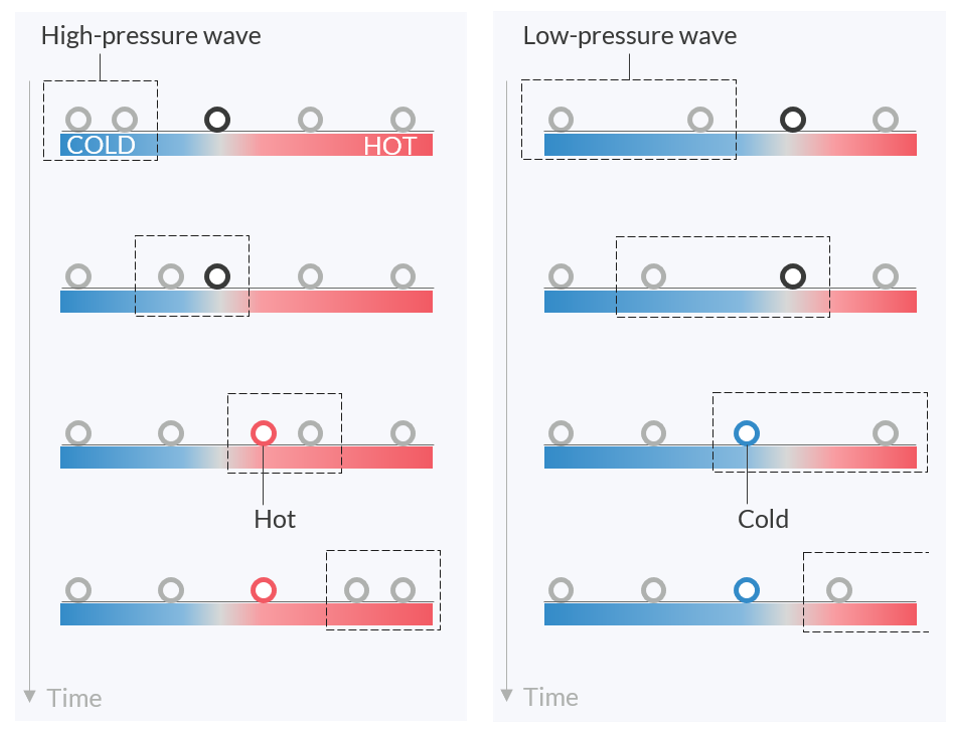
How parcels in a fluid move under a traveling wave coming from the left. An imaginary area of the wave is represented by a dotted box. With an appropriate temperature gradient in the neighboring plate, the parcel will always move to the hotter area if pushed by a high-pressure wave and move to the colder area if pulled by a low-pressure wave.
Then, consider putting a heated plate in the tube along the traveling path of the wave. If the right end of the plate is heated while the left end is kept at moderate temperature, there will be a temperature gradient in the plate. The temperature gradient heats up the parcels when the parcels move to the right, and it absorbs heat from them when they move to the left. Because a parcel is of its highest pressure when moving to the right, the heating of the parcel pushes up the maximum value of the pressure. In the same way, the heat absorption when a parcel is moving to the left decreases the minimum pressure too. Those periodic ups and downs in the temperature synchronize the movement of parcels and finally increase the amplitude of the wave. All of the parcels work together as a chain to convey the pressure wave and add an energy to the wave by the exchange of heat. Note that the temperature gradient in the plate should be in the same direction as the wave propagation, otherwise the wave will simply attenuate.
If you’re wondering if there is a device with a reversed cycle of the engine, the answer is yes, there is. This system is called a thermoacoustic heat pump or thermoacoustic refrigerator, and it can move heat by using acoustic waves. The working principle is simple: When a high-pressure wave arrives at a parcel, the parcel is compressed, the temperature consequently increases, and the parcel starts to dissipate its heat to the neighboring object while moving to the right. Conversely, with a low-pressure wave, a parcel absorbs heat and moves to the left.
The explanation here is only for introductory purposes and does not contain all of the details of thermoacoustic engines. If you’re interested in more in-depth information about thermoacoustic engines, see Ref. 2.
Linearized Equations for Thermoacoustics Modeling
It’s always important to think about what set of equations and which interface is suitable for a new simulation. For the present modeling example, it may seem reasonable to use the Acoustics Module to simulate the thermoacoustic oscillation since the phenomenon is related to acoustic waves. In addition, since the academic field is called thermoacoustic, the Thermoviscous Acoustics interface seems to be a good choice. Let’s check the equations and the capability of this interface to validate our choice.
The Thermoviscous Acoustics interface uses the following equations in a time-domain analysis:
where \rho, \bm{u}, T, and p are density, velocity, temperature, and pressure, respectively. The subscript {\cdot}_0 expresses that the value belongs to the background mean flow, while the variables with the subscript {\cdot}_t represent the acoustic perturbations. The governing equations of the Thermoviscous Acoustics interface are derived from the Navier–Stokes equations (the exact equations of fluid motion) based on the assumption that every second-order perturbation term can be omitted from the simulation and that the velocity of the background mean flow is zero (\bm{u}_0=\bm{0}).
We have to pay attention to the neglected nonlinearities and whether the linearized equations cover the phenomenon of our interest. In the case of thermoacoustic engines, the heat exchange between a fluid and a heat exchanger is expressed by the diffusion term \nabla \cdot (k\nabla T_{\rm t}), and the heat transfer due to the acoustic oscillation is expressed by the linearized advection term \bm{u}_{\rm t}\cdot \nabla T_0. A cold fluid with a high pressure advected by the term \bm{u}_{\rm t}\cdot \nabla T_0 is heated up in a heat exchanger by \nabla \cdot (k\nabla T_{\rm t}), and the energy is incremented through the third equation. These terms describe the important mechanisms of heat transfer in our system, and therefore the linearized equations seem to be a good fit for modeling the engine.
Also note that there is no advection term that stands for the coupling of the time-varying temperature field and the oscillation velocity, \bm{u}_{\rm t}\cdot\nabla T_t. This coupled representation would show the oscillation-induced transport of the transient temperature field. The advection term is important for the simulation of the heat pumps, where the temperature gradient at equilibrium is determined as a result of oscillations and not available a priori. In such cases, we can use the feature Nonlinear Thermoviscous Acoustics Contributions, which allows the model to take the nonlinear terms into account in the Thermoviscous Acoustics, Transient interface. Simulating nonlinearities can be costly, so the nonlinear functionality should only be added in the relevant domains.
Modeling in COMSOL Multiphysics®
So far, we have covered the basic working mechanisms of thermoacoustic engines and the relevant governing equations for modeling them, so let’s move on to the model building. You can access the model files for the examples shown here in the Application Gallery. As discussed in the previous section, we will use the Thermoviscous Acoustics interface to model traveling-wave thermoacoustic engines. Because the stationary background temperature field is not uniform, the Heat Transfer interface is also used. Rather than using the two interfaces simultaneously, the whole study can be split into two steps: a Stationary step for the background temperature field and a Time Dependent step for the acoustic fields. The coupling is simply done by setting the solution of the Heat Transfer interface as the equilibrium temperature in the Thermoviscous Acoustics Model node.
As for the boundary conditions of the Thermoviscous Acoustics interface, we should set the wall of the heat exchanger to be isothermal (T_{\rm t} = 0). This condition heats up the temperature of the fluid with a high pressure (where T_{\rm t} is less than zero due to the advection from the cooler area) and cools down the fluid when its pressure is low (where T_{\rm t} is higher than zero).
Example 1: Simple Loop
First, we will model an engine consisting of a simple loop. It has a heat exchanger in the right passage, and the whole passage forms a closed circuit. The stationary temperature will appear as shown in the figure below. The temperature gradient at the lower region of the heat exchanger can be eye-catching, but our focus is on the temperature gradient in the small gaps of the heat exchanger.
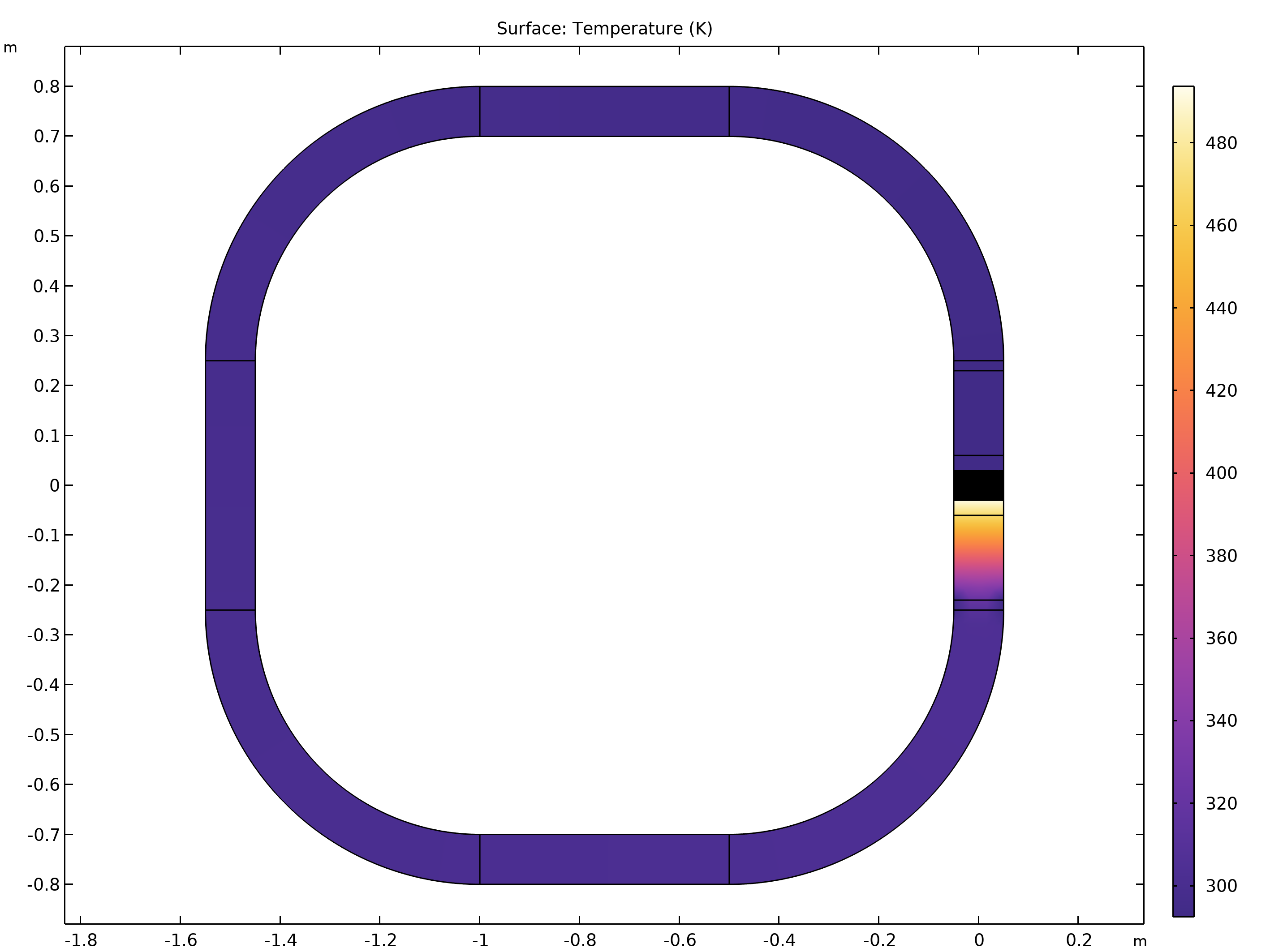
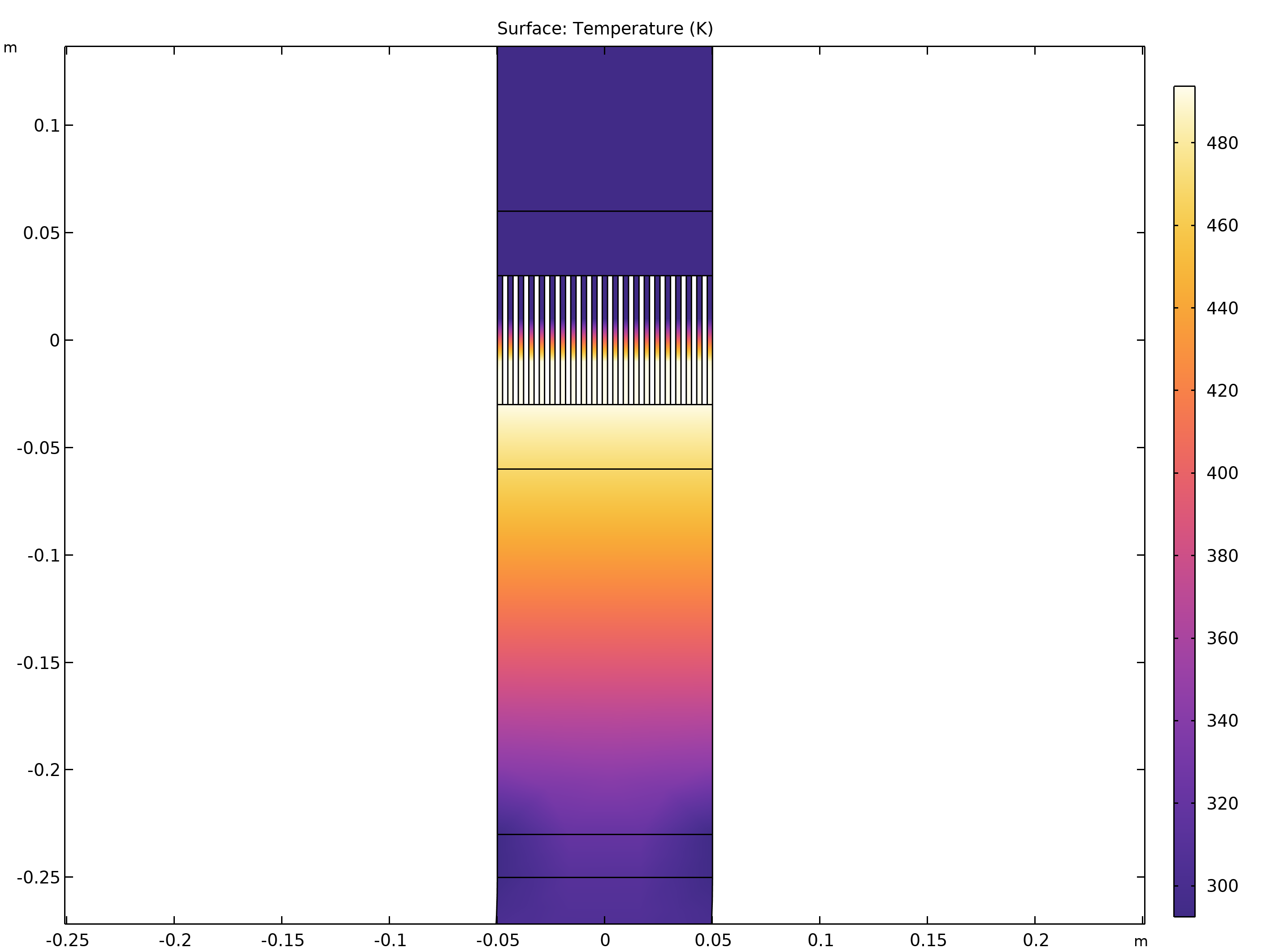
The equilibrium temperature in a simple loop-like engine (left: full system; right: close-up around the heat exchanger). The lower end of the narrow passages in a heat exchanger is heated at 493 K.
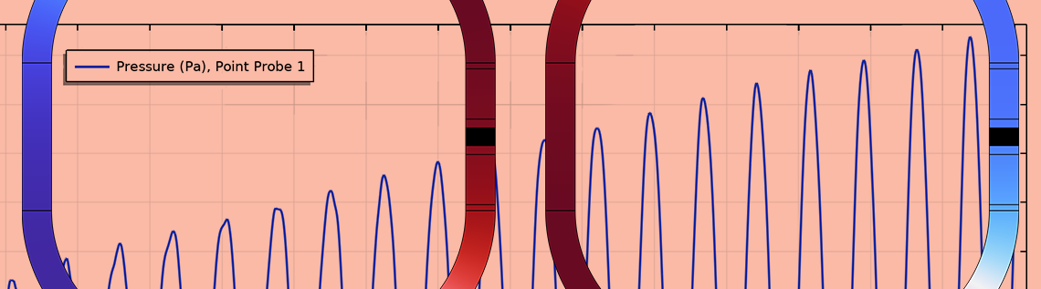
In the Time Dependent study step, a standing wave is given as the initial condition of the pressure so that it can trigger the oscillation inside the loop. As the simulation continues, the amplitude grows, as captured by the Point Probe feature (shown below). It is clear that the oscillation keeps growing, which means that the thermal energy is converted into acoustic energy.
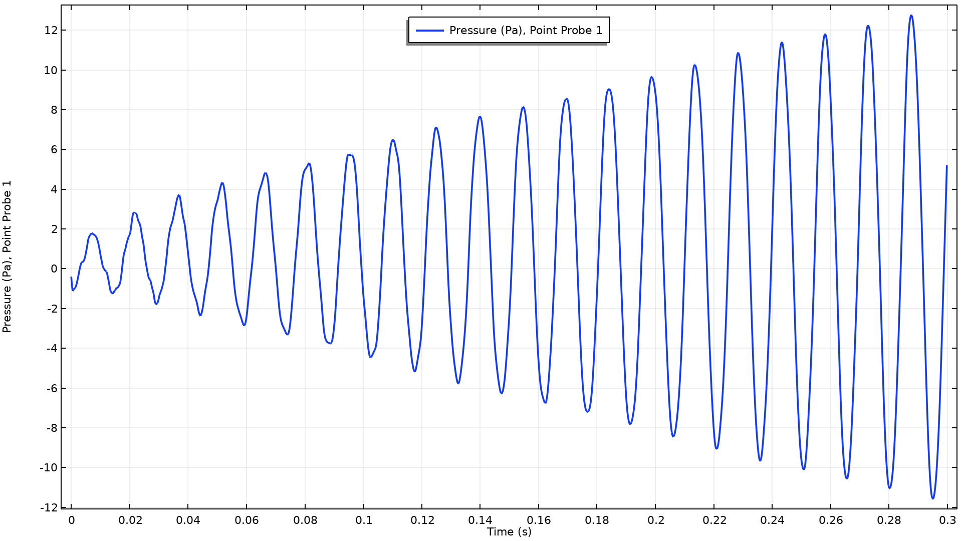
The Point Probe feature is set to track the pressure in the engine. The pressure data is taken at a point in the heat exchanger, which is close to the pressure node of the standing wave used as the initial pressure distribution.
So, what does the pressure look like in the engine? The three figures below visualize the pressure distribution at t = 0.281 s, 0.285 s, and 0.289 s, respectively. A standing wave is given at t = 0 s, but after a short period, the distribution starts to rotate in the clockwise direction. The wave travels in the same direction as the temperature gradient in the heat exchanger, and the counterclockwise component of the initial standing wave attenuates due to the lack of energy supply for it. Interestingly, the excitation of a counterclockwise wave can be simulated by flipping the direction of the temperature gradient in the middle of the simulation. In the model file, the Stationary study step is calculated again with the reversed temperature profile at t = 0.3 s, and the Time Dependent study reflects the change in the equilibrium temperature since then. The clockwise wave remains until approximately t = 0.6 s. Subsequently, a standing-wave-like distribution appears in the engine, and the wave finally propagates counterclockwise.
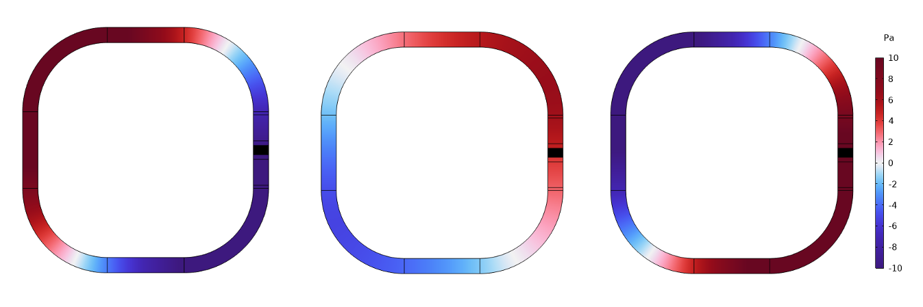
History of the pressure distribution (left: t = 0.281 s; middle: t = 0.285 s; right: t = 0.289 s). Both the high-pressure area and the low-pressure area move in the clockwise direction due to the thermoacoustic effect discussed earlier.
Example 2: Loop with a Stub
In addition to the single loop, we will check one more configuration. The following figure shows the next model example with a complex geometry. The geometry imitates the experimental setup in Ref. 3. The model is 2D and simplified to have the same hydraulic diameter of the heat exchanger discussed in the reference. The branched pipe (called stub) at the lower-right end is added for the future extraction of the acoustic energy. Like in Example 1, the loop is used in the engine to convert thermal energy into acoustic energy, but here, a portion of the energy can be extracted at the stub.
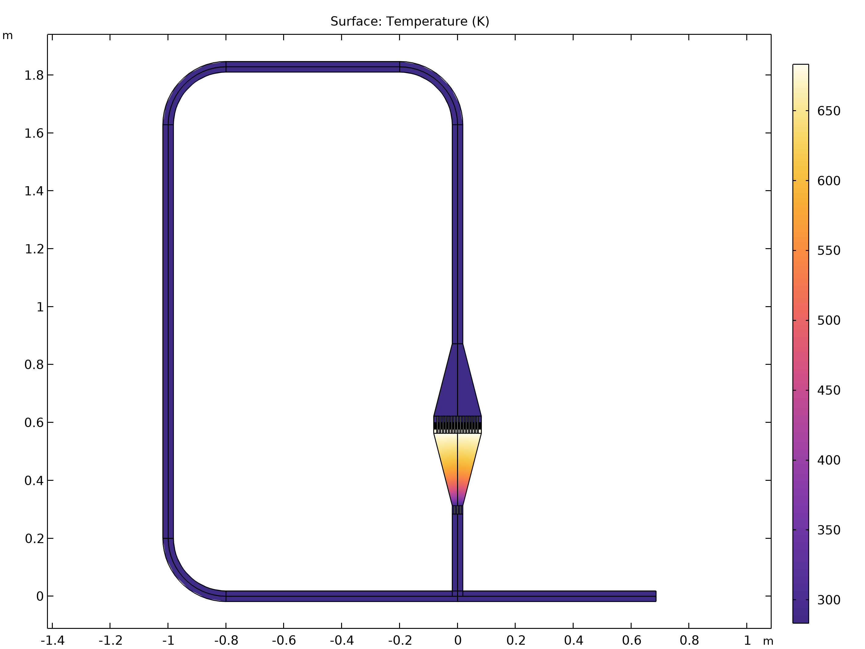
The equilibrium temperature in a model with a stub. The geometry imitates the experimental setup in Ref. 3.
The instantaneous pressure distributions in the engine are shown in the figure below. There is a sharp drop where the arc length equals 3.6 m, caused by the viscous drag in the small gaps at the heat exchanger. Notably, the amplitude of the pressure is strongly dependent on the position. This is due to the complexity of the model, such as the viscous drag and a standing-wave component sustained in the engine. In the figure, the time-wise maximum value of the absolute pressure, labeled as max(|p|), is also plotted at each position. Note that even though the amplitude seems a bit large, this simulation assumes no turbulence and that any perturbation is linear. When nondimensionalized with its spatial maximum, the distribution of the approximate amplitude, max(|p|), agrees well with the experimental and analytical data in Ref. 3.
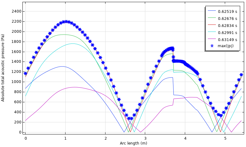
Instantaneous pressure distributions along the loop and the approximated amplitude, max(|p|), computed by a state variable.
Check Out Other Examples
Since the demonstration by Professor Rijke, there has been significant growth in the understanding of thermoacoustics, and its application in energy devices is now actively studied. In this blog post, we covered how thermoacoustic engines can be modeled using the Thermoviscous Acoustics interface, and the interesting characteristics of the engines were visualized.
In the Application Gallery, you will find many models across physical disciplines. Two models relating to thermoacoustics include:
- Simple Thermoacoustic Engine, which is a model of a standing-wave thermoacoustic engine. There are multiple model files, offering a comparison of setting up the same model with two different approaches: a linear perturbation approach by the Thermoviscous Acoustics, Transient interface and a full nonlinear approach by the Nonisothermal Flow multiphysics interface. The latter approach solves the Navier–Stokes equations and takes the nonlinearity into account at the cost of increased computational time.
- Thermoacoustic Engine and Heat Pump, which is a model of a standing-wave heat pump. Unlike thermoacoustic engines, the simulation of thermoacoustic heat pumps require the calculation of the nonlinear advection term \bm{u_t}\cdot\nabla T_{\rm t} because the temperature will keep decreasing due to the thermal transportation effect. In the model, the Nonlinear Thermoviscous Acoustics Contributions node is added to the Thermoviscous Acoustics interface to account for the nonlinearity. The model also uses the Thermoviscous Acoustic-Thermal Perturbation Boundary coupling, a new feature in version 6.2. The coupling is used to simulate the heat exchange between the oscillating fluid and the solid plates in the passage, since the solid temperature keeps decreasing in accordance with the pumping of the heat.
References
- P.L. Rijke, “LXXI. Notice of a new method of causing a vibration of the air contained in a tube open at both ends,” The London, Edinburgh, and Dublin Philosophical Magazine and Journal of Science, vol. 17, no. 116, 419–422, 1859; https://doi.org/10.1080/14786445908642701
- G.W. Swift, Thermoacoustics: A Unifying Perspective for Some Engines and Refrigerators, Springer, 2017; https://doi.org/10.1007/978-3-319-66933-5
- M. McGaughy et al., “A Traveling Wave Thermoacoustic Engine—Design and Test,” Letters Dyn. Sys. Control, vol. 1, no. 3, July 2021; https://doi.org/10.1115/1.4049528


Comments (0)