Guest blogger Kirill Horoshenkov (FREng), professor of acoustics at the University of Sheffield in the UK, discusses how to model acoustical properties of porous media using the COMSOL Multiphysics® software and the Acoustics Module.
The interest in the acoustical properties of porous media is mainly associated with the great ability of these media to absorb and modify the incident sound wave, which interacts with the fluid filling the material pores. Viscous friction, inertia, and thermal dissipation effects are responsible for the observed acoustical properties of rigid-frame porous media. These effects are controlled by the material porosity and other parameters of the pore structure. Although for a majority of practical engineering problems, the acoustical properties of porous materials are not of direct interest, the relationship between the acoustical properties, porosity, and frame morphology are of significant interest.
In applications related to energy storage, it is important to measure the porosity and tortuosity of ceramic separators, which control the electrolyte uptake by the porous separator and its ability to conduct an electrical current. In applications related to filtration operations, similar characteristics are measured routinely to determine the permeability of the membrane in the presence of a flow of fluid. In pharmaceutical applications, it is often of interest to measure the mean particle size and compaction, particle size distribution, and amount of moisture absorbed by the particle mix. In chemistry and chemical engineering applications, it is important to know the internal pore surface area of materials that are used to deliver catalysts to control the chemical reaction and convert noxious substances in chemically inert bonds. In noise control applications, it is of interest to estimate the ability of a porous layer to absorb sound.
6-Parameter Johnson–Champoux–Allard–Lafarge Model
COMSOL Multiphysics includes a range of models that can predict the acoustical properties of porous media. Historically, the Johnson–Champoux–Allard–Lafarge (JCAL) model, included in the Poroacoustics feature (Figure 1) available in the Acoustics Module, has been used for this purpose and cited rather extensively (over 2000 Scopus citations as of November 15, 2020).
The basis for the JCAL model was originally proposed in 1991 (Ref. 1). It requires 6 nonacoustical parameters to predict the complex, frequency-dependent dynamic density of the fluid trapped in the material pores
(1)
and its dynamic compressibility
(2)
Figure 1: Screenshot of the Settings window for the Poroacoustics interface, illustrating settings for the original six-parameter JCAL model.
The physical meaning of these equations is well explained in the COMSOL documentation and on the APMR portal run by Matelys. In the above equations, the key nonacoustical parameters that control the acoustical properties of porous media are:
- Porosity, \epsilon_p
- Viscous flow resistivity, \sigma
- Thermal flow resistivity, \sigma’
- Viscous characteristic length, \Lambda
- Thermal characteristic length \Lambda’
- Tortuosity, \alpha_\infty
\Lambda is a measure of the pore scale at which the viscous and inertia effects are particularly pronounced. \Lambda’ is the pore scale where the thermal dissipation effects are particularly pronounced. \alpha_\infty is a measure of the twistedness in the pore and complexity of the path that the sound wave takes while propagating through the porous layer. Often, the viscous and thermal flow resistivities are replaced with their static permeability counterparts, i.e., \kappa_0=\mu / \sigma and \kappa_0’=\mu / \sigma’, respectively. The other parameters in the above equations are standard and known:
- The equilibrium density of fluid, \rho_f
- i = \sqrt{-1}
- The angular frequency of sound, \omega
- The dynamic viscosity of the fluid, \mu
- The Prandtl number, N_\textrm{Pr}
Key acoustical properties of a porous medium are the characteristic impedance and wave number defined as
(3)
respectively.
Editor’s note: COMSOL uses a slightly different notation. Please see the “About the Poroacoustics Models” section of the Acoustics Module User’s Guide in the documentation.
It is unusual to directly measure the characteristic impedance and wave number, although experimental methods for measuring these quantities do exist, e.g., the three-microphone impedance tube method proposed by Doutres et al. (Ref. 2) However, at present, there is no agreed standard method to measure z_b and k_b directly. The most popular ISO standard laboratory method adopted worldwide to measure the acoustical properties of porous media is to use a two-microphone acoustic impedance tube (Ref. 3). According to this standard, the complex reflection coefficient
(4)
and normalized surface impedance
(5)
of a hard-backed layer of an acoustic material with thickness h can be measured in a frequency range, which is limited by the diameter of the tube and spacing between the two microphones (see section 4.2 in Ref. 3).
Here, c_0 is the speed of sound in the fluid. Usually a model is fitted to measured surface impedance or reflection coefficient data through a parameter inversion (Ref. 4) or some other fitting procedure.
Editor’s note: This tutorial model of an impedance tube details how to estimate parameters via data generation.
It has been shown that the JCAL model works well through a parameter fit for a wide range of porous media with arbitrary pore geometry and pore size distribution, e.g., in the case of fibrous materials (section IV in Ref. 5), granular media (Ref. 6), and foams (section V in Ref. 7). The question is how to measure without fitting and to accurately assign the values of the six parameters that are required by the JCAL model to predict the acoustical properties of a particular material that may not not be well characterized. Although it is relatively straightforward to determine the porosity and viscous flow resistivity nonacoustically, measuring the viscous characteristic length, \wedge; thermal characteristic length, \wedge’; and thermal permeability, k_0′ is far from simple and requires a highly sophisticated laboratory setup. Similarly, it is not easy to measure the tortuosity, \alpha_\infty. As a result, these four parameters are rarely measured and usually guessed or inverted from fitting to data.
From a 6- to 3-Parameter JCAL Model
More recently, Horoshenkov et al. (Ref. 8–9) proved that the use of more than three parameters in the JCAL model is not necessary at all. The authors presented theoretical (Ref. 8) and experimental (Ref. 9) evidence that the surface acoustical impedance of a range of porous media with pore size distribution can be predicted through the knowledge of the three directly measurable nonacoustical parameters only:
- Porosity, \epsilon_p
- Median pore size, \bar{s}
- Standard deviation in the pore size, \sigma_s
It was shown that
and
This approach effectively halves the number of parameters required to predict the acoustical properties of porous media very accurately. The new model is well suited for using acoustical data for measuring and inverting key nonacoustical properties of a wider range of porous media used in a range of applications that are not necessarily acoustic. The authors also suggested a new theoretical model (Padé approximation) for the bulk dynamic density and compressibility of the fluid in the material pores (Ref. 8), which is included as of COMSOL Multiphysics version 5.6.
Selecting a 3-Parameter Model in COMSOL Multiphysics®
Figure 2 presents a screenshot showing how to choose the new three-parameter model in the Poroacoustics feature in the Pressure Acoustics, Frequency Domain interface in COMSOL Multiphysics as of version 5.6. This model choice requires the knowledge of the material porosity, \epsilon_p (dimensionless), median pore size, \bar{s} [m], and standard deviation in the pore size, \sigma_s [\phi-units] (Ref. 8). Appropriate values of these parameters can be selected using the bottom part of the Poroacoustics settings, as shown in Figure 2.
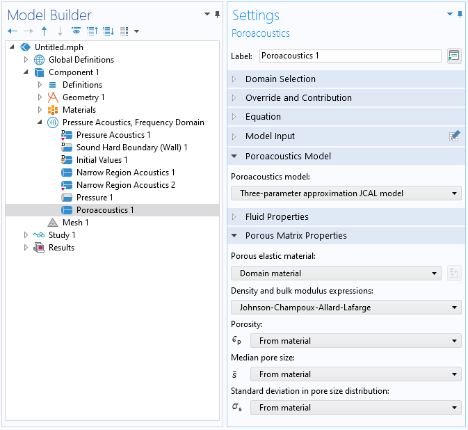
Figure 2: Screenshot of the Poroacoustics interface, illustrating settings for the new three-parameter model.
In order to use this three-parameter model, choose Three-parameter approximation JCAL model in the Poroacoustics feature. The Poroacoustics feature will use either the original JCAL equations for the dynamic density and compressibility (Eqs. 1–2) or new equations for these quantities proposed in Ref. 8. This choice can be made via the density and bulk modulus expressions. In order to use the original JCAL equations, select Johnson–Champoux–Allard–Lafarge. Otherwise, select the Padé approximations proposed in Ref. 8. This choice of the equations for the dynamic density and compressibility does not make much of a difference to the prediction, except the Padé approximation more closely matches the true low-frequency behavior of the equivalent fluid in a porous media with cylindrical pores Ref. 8.
Figure 3 shows the measured normalized surface impedance spectra, z_s(\omega), for a hard-backed 16.5-mm layer of melamine foam. This figure also shows the predictions made with the original JCAL model (dashed lines) and with the model proposed in Ref. 8 (solid lines) for the same set of parameters: \epsilon_p=0.998, \bar{s}=115 \mum, and \sigma_s=0.234 \phi-units. The two sets of lines are almost indistinguishable and accurate within 4%, which is better that the usual reproducibility of the impedance tube experiment (5%).
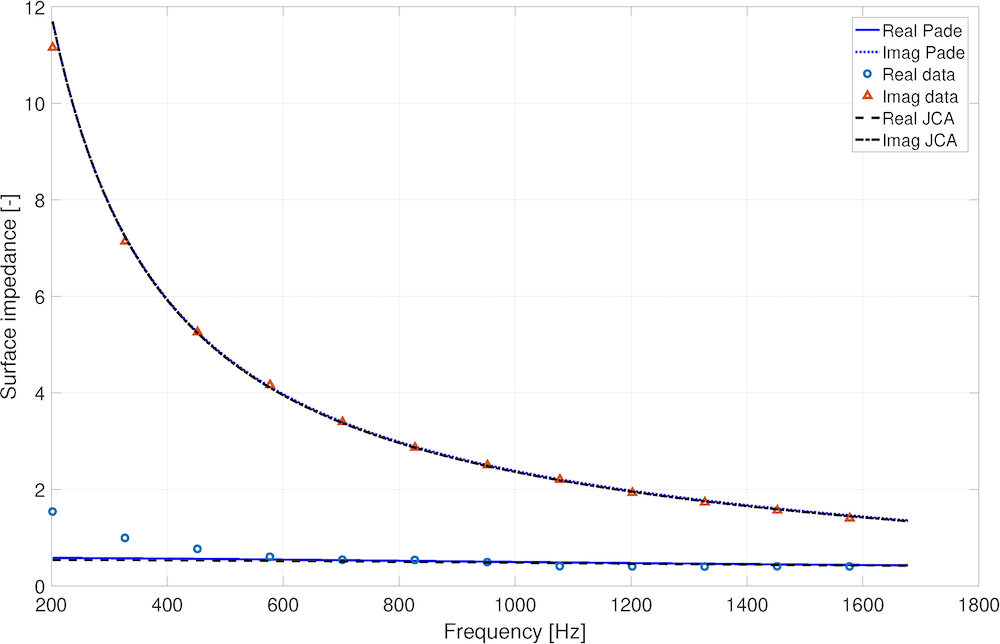
Figure 3: A comparison of the normalized measured and predicted complex surface impedance spectra for a 16.5-mm layer of melamine foam, which is hard backed.
Example Application of the 3-Parameter Model
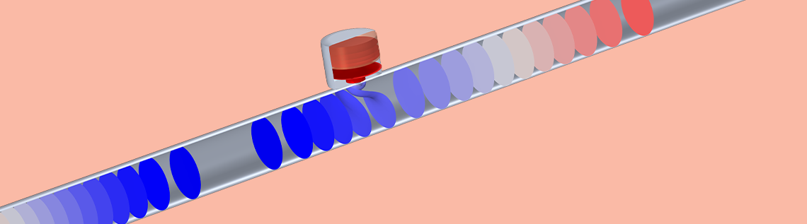
It may be of interest to look at an application of this model. Let us consider a 25-mm diameter waveguide loaded with a Helmholtz resonator branch in the middle of it. The resonator has a porous lining to increase its damping. The lining is a 21.5-mm layer of felt with the following parameters: \epsilon_p=0.998, \bar{s}=147 \mum, and \sigma_s=0.325 \phi-units. This problem is illustrated in Figure 4.
The first question is: What would be the absorption, reflection, and transmission coefficients for sound propagation in the presence of this resonator? The other question is: Will the COMSOL Multiphysics simulations based on the JCAL and Padé approximation models to predict the acoustical properties of felt return similar results? Figure 4 presents the results of this simulation, which illustrate that for this particular problem, the predictions by the two models are almost identical. The parameters for felt used in this model make good physical sense because these have been validated via a nonacoustical experiment (Ref. 9).

Figure 4: COMSOL Multiphysics model of a waveguide with a Helmholtz resonator branch.

Figure 5: A comparison of the predicted reflection, transmission, and absorption coefficient spectra through a waveguide with a Helmholtz resonator branch.
Try It Yourself
Try modeling the Helmholtz resonator with a porous layer featured in this blog post by clicking the button below.
References
- Champoux, Y. and Allard, J.-F., “Dynamic tortuosity and bulk modulus in air-saturated porous media”, Appl. Phys., vol. 70, no. 4, pp. 1975–1979, 1991. https://doi.org/10.1063/1.349482
- Doutres, O., Salissou, Y., Atalla, N., Panneton, R. “Evaluation of the acoustic and non-acoustic properties of sound absorbing materials using a three microphone impedance tube”, Acoust., vol. 71, no. 6, pp. 506–509, 2010. http://dx.doi.org/10.1016/j.apacoust.2010.01.007
- ISO 10534-2:1998, “Determination of sound absorption coefficient and impedance in impedance tubes, Part 2: Transfer-function method”, International Organization for Standardization, Geneva, Switzerland, 1998. https://www.iso.org/standard/22851.html
- Horoshenkov, K. V., “A Review of acoustical methods for porous material characterisation”, J. Acoust. Vib., vol. 22, vol. 1, pp. 92–103, 2017. https://doi.org/10.20855/ijav.2017.22.1455
- Allard, J.-F. and Champoux, Y., “New empirical equations for sound propagation in rigid frame fibrous materials”, Acoust. Soc. Am., vol. 91, no. 6, pp. 3346–3353, 1992. https://doi.org/10.1121/1.402824
- Allard, J.-F., Henry, M. Tizianel, J., Kelders L. and Lauriks, W., “Sound propagation in air-saturated random packings of beads”, Acoust. Soc. Am., vol. 104, no. 4, pp. 2004–2007, 1998. https://doi.org/10.1121/1.423766
- Perrot, C., Chevillotte, F., Hoang, M. T., Bonnet, G. BÃl’cot, F.-X., Gautron, L. and Duval, A., “Microstructure, transport, and acoustic properties of open-cell foam samples: Experiments and three-dimensional numerical simulations”, Appl. Phys., vol. 111, no. 014911, 2012. https://doi.org/10.1063/1.3673523
- Horoshenkov, K. V., Groby, J.-P., and Dazel, O., “Asymptotic limits of some models for sound propagation in porous media and the assignment of the pore characteristic lengths”, Acoust. Soc. Am., vol. 139, no. 5, pp. 2463–2474, 2016. https://doi.org/10.1121/1.4947540
- Horoshenkov, K. V., Hurrell, A. and Groby, J.-P., “A three-parameter analytical model for the acoustical properties of porous media”, vol. 145, no. 4, pp. 2512–25178, 2019. https://doi.org/10.1121/1.5098778
Acknowledgement
Model geometry and parameters are courtesy of Alexander J. Dell, Department of Mechanical Engineering, The University of Sheffield, UK.
About the Author
Kirill Horoshenkov (FREng) is professor of acoustics in the Department of Mechanical Engineering at the University of Sheffield, UK. He graduated from Moscow University for Radioengineering and Automatics, Russia, in 1989 with an MEng in electroacoustics and ultrasonic engineering. In 1997, he obtained a PhD in acoustics from the University of Bradford, UK. He has a track record of applying his acoustic expertise to a range of engineering problems, including outdoor sound propagation, acoustics of porous media, and acoustic sensing with robotics. He leads the EPSRC Programme Grant Pipebots and EPSRC UK Acoustics Network with over 1000 members. He published over 90 refereed journal papers and a similar number of papers in conference proceedings. He is an author or coauthor of 10 patents/patent applications. Three patents that bear his name or his direct contribution have been exploited commercially by Acoutechs Ltd (acoustic material manufacturing taken over by Armacell), Acoustic Sensing Technology Ltd (acoustic inspection for buried pipes), and nuron Ltd (fiber-optic cable sensing of buried pipes).


Comments (0)