

In a previous posting, we looked at computing and controlling the volume of a cavity filled with an incompressible fluid, which solved for the static deformation of a fluid-filled rubber seal. In that example, we did not explicitly model the fluid, but added an equation to solve for the pressure, assuming incompressibility of the fluid. Here, we will extend this approach and include the hydrostatic pressure of the fluid in the deforming container.
Squeezing a Water Balloon
Consider a rubber balloon, completely filled with water and resting on a surface within a hole, while being pushed from the top by an indenter. The deformation of the balloon is due to the weight of the fluid as well as the indenter pushing down from the top, see below. The rubber material is modeled with a hyperelastic material model. We will use the technique explained in the previous entry to keep the volume of the cavity constant as it deforms.
The deformation of the balloon is due, in part, to the weight of the fluid, which causes it to bulge outwards and into the depression. It also deforms due to the compression from above, which causes it to bulge outwards and upwards. As a consequence of this compression, the depth of the fluid inside the balloon will change. We want to solve for this change in depth without having to solve the Navier-Stokes equations for the fluid flow, since we are only interested in the static (time-invariant) solution.
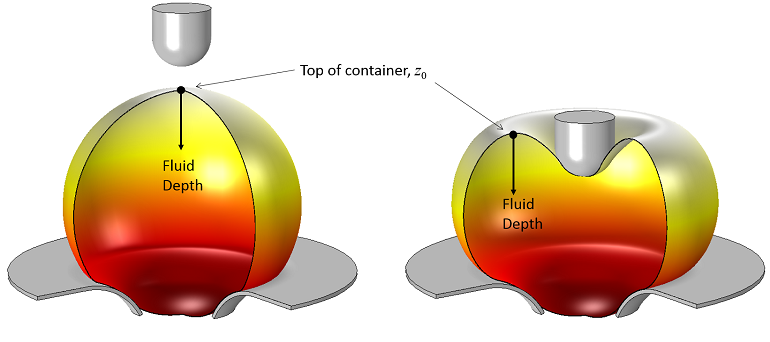
A rubber balloon filled with water is compressed at the center. As the balloon is squeezed, the location of the highest point and the depth of fluid changes, altering the hydrostatic pressure distribution.
Incorporating Hydrostatic Pressure
A container of fluid will exert a hydrostatic pressure on its walls:
where \rho is the density of the fluid, g is the force of gravity, z_0 is the location of the top of the container, and p_0 is the pressure of the fluid at the top of the container. Since the balloon is filled with an incompressible fluid, the pressure, p_0, will increase as we squeeze it with the indenter.
We can also see, from the image above, that the depth of the fluid changes as the balloon is compressed. Furthermore, it appears as if computing the depth requires knowing the location of the top and bottom of the container. So, how do we incorporate this change in depth? Let’s find out…
As shown below, there are two components to the pressure loads applied inside the balloon. The first part of the load is computed from the Global Equation. The second pressure load is due to the hydrostatic pressure. Ideally, this second pressure load would be based upon the depth of the fluid, but this depth is a variable that we don’t know. So instead, let’s enter a hydrostatic load based only upon the z-location, which could have an arbitrary zero level.
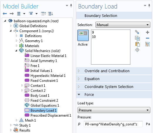
The applied pressure load on the inside boundary of the balloon is the sum of the pressure load computed by the Global Equation and the hydrostatic pressure. The hydrostatic pressure is ramped up during the solution.
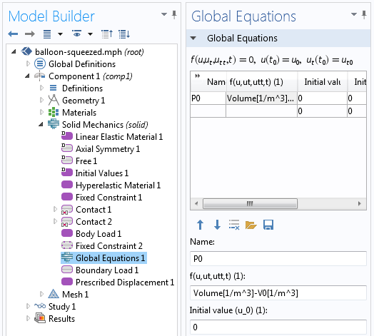
The Global Equation constrains the volume to remain constant during deformation.
So, it appears here as if we are applying a pressure load to constrain the volume and a load that is directly proportional to the z-location, but we are not correctly computing the hydrostatic pressure, since we do not know z_0. As it turns out, however, the Global Equation does a little bit more than you might first expect.
To see this, let us slightly re-write the equation for the pressure inside the balloon:
We can see right away that this almost exactly matches the equation we entered as the pressure load, p(z)= P_0-\rho g z, except that the pressure we are computing via the global equation is the pressure at the top of the container plus an offset due to the unknown z-location of the top. So, although we are only solving for a single additional variable, P_0, it accounts for two physical effects: the change in pressure due to the volume constraint as well as the change in the z-location of the top of the fluid.
Since this model contains both geometric and material nonlinearities and a nonlinearity due to the contact, converging to the solution can be difficult. To address this, we will use load ramping to slowly increase the effect of gravity on the model, and to gradually squeeze the balloon. A 2D-axisymmetric model is used to exploit the symmetry of the structure.
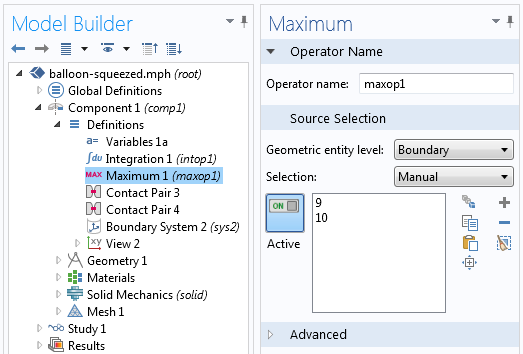
The Maximum Coupling Operator is used to find the highest point inside the cavity for postprocessing.
After we solve the model, we can postprocess the magnitude of the hydrostatic pressure by using the Maximum Coupling Operator to compute the maximum z-location along the inside boundary of the balloon.
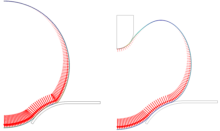
The solution where the arrows indicate the hydrostatic pressure load that varies with depth.
The plot above shows the hydrostatic pressure load on the inside of the balloon. The length of the arrows is given by the expression: WaterDensity*g_const*(maxop1(z)-z), where maxop1(z) gives the z-location at the top of the deformed cavity.
Concluding Remarks
In this example, we have modeled the varying depth of a fluid in a deformable container (a balloon, in this case). The Global Equation that is used to solve for the fluid pressure that keeps the volume constant also accounts for the change in the depth of the fluid as the balloon deforms.
By using this approach, we solve a fluid-structure interaction problem without explicitly having to solve the Navier-Stokes equations, thus saving significant computational resources. If you are interested in this type of modeling, or would like more details about this model, please contact us.


Comments (11)
Christoph Kübler
June 6, 2014Hi, is it possible to test this modell ?
Best regards
Christoph Kübler
Amir Shemer
September 6, 2018Hello!
I also want to get this file for testing and training.
Thanks.
Amir Shemer.
Walter Frei
September 11, 2018 COMSOL EmployeeHello,
Although the model for this blog is not available, the key point of this blog is primarily only to introduce the usage of the global equation in concert with the component coupling operator, the implementation of which should follow the screenshots and directions show here. Of course, if you’re having technical questions, please reach out to our support team, support@comsol.com.
Aero Aero
September 19, 2018Hello,
It is written in this article that since the balloon is filled with an incompressible fluid, the pressure, p_o will increase as we squeeze it with the indenter. Could someone please explain why that is the case? TIA,
-aeroaero
Walter Frei
September 20, 2018 COMSOL EmployeeHello Aero,
That is a good point, it does not matter if the fluid is incompressible or not, the pressure will increase due to the load.
Amir Shemer
September 27, 2018Hello Walter,
The main question is how to set the pressure of a liquid or air in a closed volume?
Thanks,
Amir Shemer
Amir Shemer
September 27, 2018For example, there is a human eye, and we want to model the measurement of intraocular pressure in it. How to set the initial pressure?
Amir Shemer
Walter Frei
September 27, 2018 COMSOL EmployeeHello Amir,
The point here, and more explicitly in this previous article:
https://www.comsol.com/blogs/computing-controlling-volume-cavity/
is that you do not need to compute the pressure, the software does so for you, under (in this case) the assumption of an incompressible fluid. In the previous blog, the case of a compressible fluid is also discussed.
The example which you are describing, though, sounds a bit outside the scope of this article, and may be best addressed directly with the COMSOL Technical Support Team (support@comsol.com)
Amir Shemer
September 29, 2018Hello Walter,
Thank you very much for the help.
Amir Shemer
Sharique Nomani
January 1, 2021Hey, can you please tell me how you defined the volume of the cavity? I tried integrating with the intop1 operator (selected the boundary of the hyper-elastic material and computed with revolving geometry on), but intop1(1) gives the boundary area. If I select the domain of the balloon, it would give the volume of the material, which we don’t want, right? I’m a beginner so can you help me out?
中汉 林
September 9, 2021Hello Walter,
I am new to COMSOL and I want to rebuild this model. How do you calculate the volume of the water? I followed the instruction of this blog: https://www.comsol.com/blogs/computing-controlling-volume-cavity/ and set the Volume = VolumeInt(-r*solid.nr). In the function VolumeInt, I choose the inner boundary and click the computed with revolving geometry on. Then get an error: Undefined variable solid.nr. Can you help me?
Best regards,
Lin