
There are many situations where you may be interested in modeling periodic, albeit nonsinusoidal, electrical signals for the purposes of computing the resultant electric fields, thermal losses, and temperature change. As one example, electrical pulse trains can be applied to human tissue for the purpose of neuromodulation, electroporation, or thermal ablation. Although such signals can be simulated via time-domain modeling, it’s also possible to efficiently compute the linear response via a Fourier transform approach. Let’s learn more!
Table of Contents
- Introduction
- Understanding the Frequency Content of the Input Signal
- Solving in the Frequency Domain
- Reconstructing the Transient Results
- Using the FFT Results for Thermal Analysis
- Changing the Pulse Type and Spacing
- Ignoring Capacitive Effects for Further Simplification
- Closing Remarks
Introduction
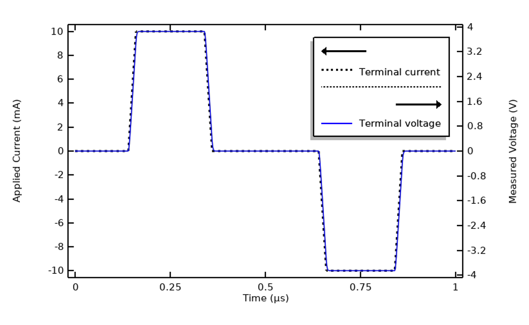
We will continue working with the example model that we used in our previous blog post, “Understanding the Transient Electromagnetic Excitation Options”, and solve it using the Electric Currents interface. (This interface is highlighted in our previous blog post and shown to be sufficient for solving this type of model.) The current excitation is a trapezoidal pulse waveform of 1 µs period. This model can be solved in the time domain. The terminal voltage and total losses within the model are shown below.
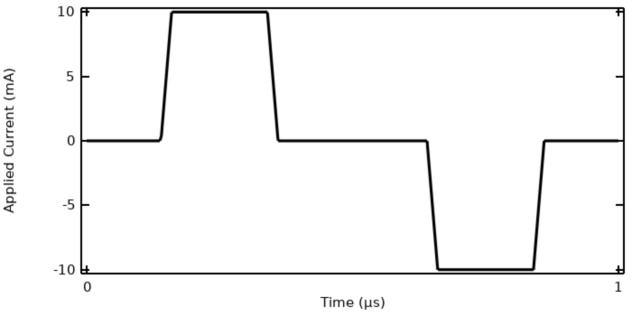
The applied current to the model, a ramped trapezoidal pulse wave.
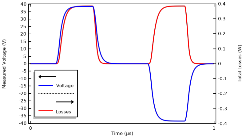
Computed terminal voltage and losses within the material over one period.
We can also extend the model to solve for the temperature and make the electric conductivity a function of temperature, thereby turning it into a bidirectionally coupled multiphysics model. The expression we will use is \sigma (T) = 0.03\exp \left(-\frac{T-20^\circ \text{C}}{20\text{K}}\right) \text{S/m}.
A fixed temperature boundary condition is applied along the side and bottom of the modeling domain. The model is solved for a single time period (1 µs), and the temperature changes over this period can be examined. As seen in the image below, the temperature change is minimal.
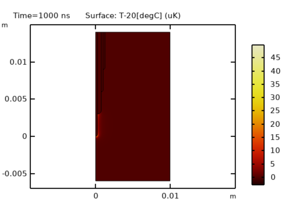
The computed temperature change after 1 µs is small.
We will, however, want to solve for a temperature variation over much longer timespans than one period, and for that this modeling approach is going to be too computationally expensive. We will need to look to other approaches. Before we get to that, though, there are several remarks to make about this model and the results:
- The applied current varies around a cycle-averaged value of zero, so the input signal has no DC component.
- The computed terminal voltage and losses go to zero between the pulses.
- Neither the electric conductivity nor the relative permittivity depends directly on the electric field.
- The terminal voltage lags the current, meaning that the system has significant capacitance.
- The rise in temperature over one period of excitation is very small.
As a consequence of the observation that the temperature rise is very small over a timespan similar to the electrical excitation period, we can treat the electrical problem as locally linear in time. This allows us to reproduce the results by instead taking the Fourier transform of the applied signal, then solving a frequency-domain model and using an inverse Fourier transform to reconstruct the transient results for the electrical model. This quickly gives us information about which harmonics of the input signal contribute significantly to the heating.
Solving for the transient temperature variation over a timespan much longer than the excitation period can be accomplished with a bidirectionally coupled model that solves for the temperature field along with several Electric Currents interfaces, one for each significant frequency component of the input signal. This will be much more computationally efficient. There are several steps to this modeling approach, as described in our Learning Center articles “Understanding Periodic Signals and Their Frequency Content”, “Using the Inverse Fast Fourier Transform to Reconstruct a Transient Signal”, and “Setting Up and Solving Electromagnetic Heating Problems”. We’ll summarize these steps here.
Understanding the Frequency Content of the Input Signal
Starting with a periodic signal, we can take the fast Fourier transform (FFT) of the signal to examine its frequency content, which can be done in terms of the magnitude of each harmonic, as well as in terms of the cumulative sum up to the current harmonic. In the figures below, the image on the left is a plot of the frequency content of a trapezoidal pulse wave and the image on the right is of the cumulative sum.


The frequency content of a trapezoidal pulse wave (left) and in terms of cumulative sum (right).
What we can see from such a preliminary step is that, at least for this example, only a relatively low number of harmonics contribute most of the energy in the signal, and certain harmonics have negligible contribution.
Solving in the Frequency Domain
Along with the FFT of the applied signal, we also need to compute the response of the system to a frequency-domain excitation, with an excitation of the same magnitude at all frequencies. Note that this does not imply that the response of the system will be equivalent at all frequencies, a topic covered in depth in our blog post “Understanding the Excitation Options for Modeling Electric Currents”. The results of sweeping over a range of frequencies is shown below in the plot of cycle-averaged losses, from which we can deduce that the model we’re working with has an impedance that varies significantly with frequency. In this case, we will solve for the first 100 harmonics, and once we know which frequencies are important, we can run a smaller set of frequencies.
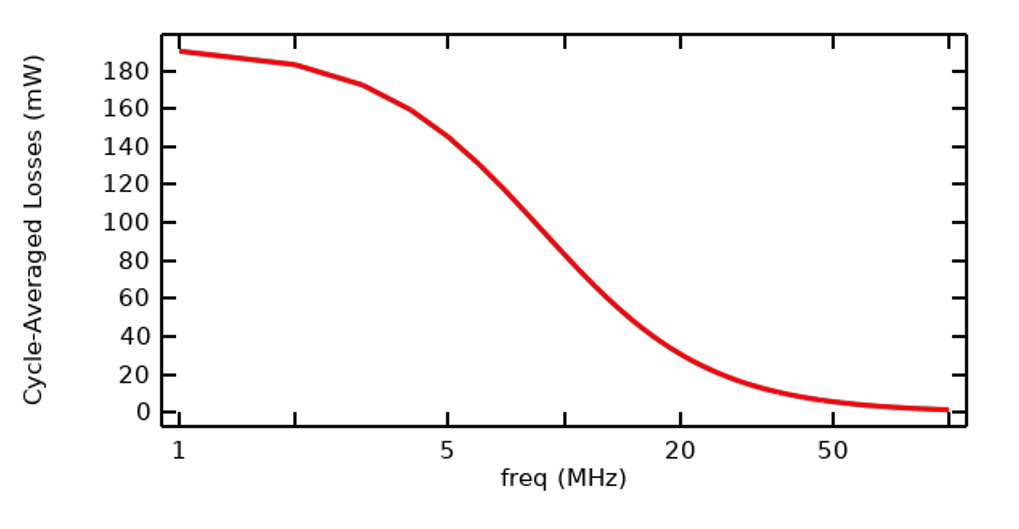
Plot of cycle-averaged losses within the sample as a function of frequency, with equivalent excitation at all frequencies.
Reconstructing the Transient Results
Since we already have the FFT of the input signal, once we have computed the frequency-domain results, with a unit excitation over all considered frequencies, we can use the inverse fast Fourier transform (IFFT) to reconstruct the transient response of the system. The plot below shows excellent agreement, and the IFFT approach is less computationally intensive.
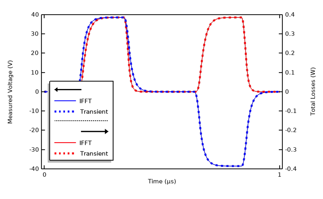
Comparison of transient results and results of reconstruction via IFFT using 100 harmonics.
Although getting excellent agreement in terms of the transient results can be useful, we are often only interested in the heating, so rather than evaluating the IFFT results in terms of their agreement in the time domain, it’s also useful to compare the time-integrated losses over one cycle. For this applied signal, 99% of the losses are captured by solving for only the first, third, seventh, and ninth harmonics. That is, the total integrated losses agree quite well even though the transient results are noticeably different.
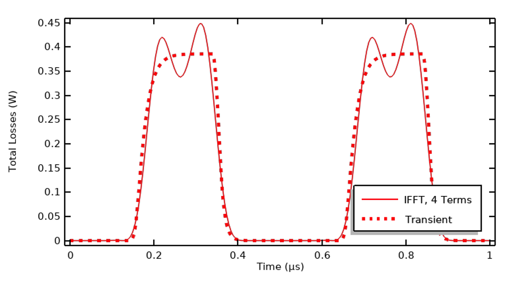
Comparison of losses in the time domain and the losses reconstructed via the IFFT using only four harmonics.
In the figure above, we can see that although agreement does not look as good, the integral of the losses over the entire time period agrees within 1%.
Using the FFT Results for Thermal Analysis
So far, we have looked at how to reconstruct the variation of the transient losses over a single period, but for the purposes of thermal analysis we are likely interested in modeling much longer times since the temperature changes occur over timespans many times longer than the period of the electrical signals. If we have materials where the electric conductivity varies with temperature, we will want to include this bidirectional coupling between the physics in our model. If we tried to solve for the electric fields and the temperature fields at the same time, with a fine-enough temporal resolution to capture the electrical excitation, then we would end up with a model that would take a very long time to solve. Although that is sometimes justified, we often want a faster approach, and that is where the data that we’ve computed so far will become very useful.
As shown below, the time-domain losses can be approximated as uniform in time, based on a sum of contributions from the first few harmonics. This is valid under the assumption that the thermal timescales are much longer than the electrical period.
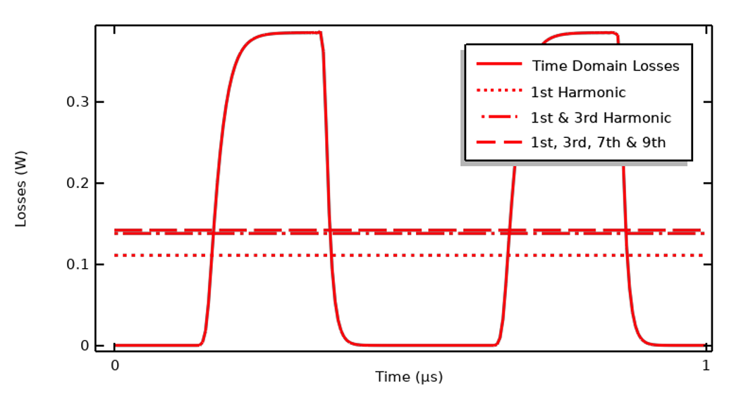
Plot comparing the time-domain losses and sum over the cycle-average computed over several harmonics.
As we observed earlier, for this input signal we only need the fundamental, third, seventh, and ninth harmonic to capture 99% of the heating over one period. This means we can set up a new model with four different Electric Currents physics interfaces, each solved in the frequency domain for a different harmonic, and multiply the magnitude of the applied current for each harmonic by the corresponding Fourier coefficient of the input signal. These interfaces can then be solved along with a transient (or stationary) thermal model, which will compute the temperature variation and incorporate the bidirectional coupling that arises since the electrical material properties are functions of temperature. This approach is relatively much more computationally efficient and allows for modeling a 3D geometry. For a guide to setting up such models where the results of an FFT of the input signal are used to define the heat loads, see our Learning Center article “Setting Up and Solving Electromagnetic Heating Problems”.
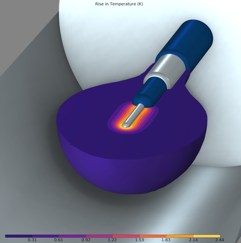
Rise in temperature computed in a 3D model, using the cycle-averaged heating due to a sum of harmonics of the applied current waveform.
Changing the Pulse Type and Spacing
It’s also worth addressing what will happen if we want to model a pulse train, a signal that is strictly positive. This signal has a DC component, which theoretically makes the IFFT more involved since we also need to consider the stationary solution. But since we are only concerned with the heating, and if the losses drop to zero between the pulses, then the sign of the excitation doesn’t matter. That is, electrical heating is the same regardless of the direction of current flow. If the heating over time drops to zero between the pulses, then there is no DC component to the heating that needs to be considered in the IFFT. So, even when dealing with an input signal that is strictly positive, it can be reasonable to instead treat it as a signal that switches from positive to negative, solely for the purposes of simplifying the IFFT reconstruction. The signal below and the previously presented signal are identical in terms of their computed losses.
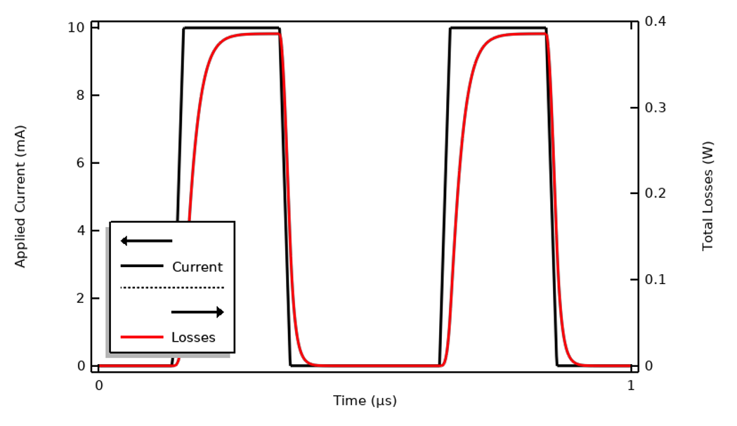
An input signal that is strictly positive will have an identical heating compared to a symmetric signal, as long as the heating profile goes to zero in between.
Let’s also change the spacing between the pulses. This increases the period of the input signal, so we might think that we need to redo the FFT. However, since the heating drops to zero between the pulses in our original signal, adding more time during which the heating is zero doesn’t alter the losses due to a single pulse. That is, if we have a pulse train with a long time period between the pulses, it’s sufficient to take the FFT of a signal with less time between the pulses, as that is sufficient to accurately predict the heating profile and it saves some computational effort. When solving the bidirectionally coupled thermal problem, the applied signal has to be scaled down by a factor of the square root of the duty cycle. In the figure below, the pulses have equivalent duration but the period is doubled, so the duty cycle is 0.5.
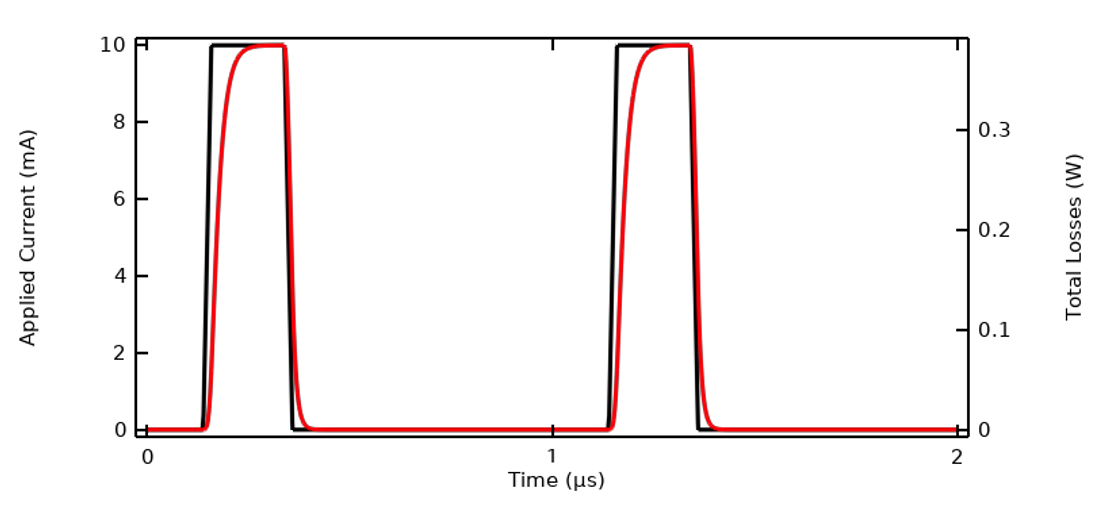
Increasing the time between pulses does not alter the heating profile of each pulse.
Ignoring Capacitive Effects for Further Simplification
The example we have considered so far was designed (in terms of materials properties and waveform) to illustrate a case where the FFT approach is the most useful. This level of complexity is not always needed. Let’s return to our first plot of applied current and terminal voltage and recreate it with a different sample material, one with an electric conductivity that is ten times greater. That will result in a response similar to the figure below. There is negligible lag between voltage and current relative to the period, meaning that there are almost no capacitive effects present. Or: The system impedance is nearly purely resistive and constant over the frequency range of interest. Similarly, if the same waveform shape was used but was ten times slower, the response would look similar.
Changing the electric conductivity to be ten times larger will alter the system response. The capacitive effects are now negligible.
Assuming that we are dealing with a nearly purely resistive system, and under the assumption that the electric conductivity is constant with respect to the frequency content of the applied signal, it’s possible to simplify the electrical model down to a stationary DC problem and thus entirely ignore the capacitive effects and resultant displacement currents. The Electric Currents physics interface can then be solved in the Stationary form, and the applied DC signal is the square root of the cycle average of the square of the transient signal:
This expression is the same regardless of whether the excitation is in terms of current, voltage, or terminated voltage. It’s valid to use this simplification as long as the electrical properties are constant with respect to frequency and electric field strength.
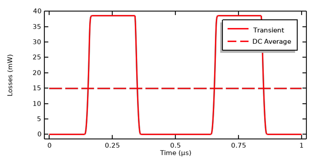
Time-domain losses for a nearly purely resistive material and the DC equivalent average.
Closing Remarks
We have looked at how to model an electrical excitation that is periodic and how this can often be reduced to consider a single period. By taking the FFT of the input signal, it’s possible to identify the important frequency content, and the transient system response can be predicted via a combination of solving for a set of frequencies and an IFFT study step.
The results of this FFT and IFFT can be used to predict the response over time and can be used as inputs to an electrothermal heating simulation. It can be especially efficient to approximate a periodic signal as a sum of several harmonics, which allows us to treat this as a bidirectionally coupled multiphysics problem in a very efficient manner. For some problem types, we can further simplify by ignoring the frequency content altogether.
If you’re modeling in this field, you’ll want to be fully aware of all of these complexities and simplifications as you build your multiphysics models.


Comments (2)
Abid Hussain
June 5, 2024Hi,
I could not find the .mph file for this tutorial.
If possible, can you provide the COMSOL file for this specific tutorial.
Thanks
Walter Frei
June 5, 2024 COMSOL EmployeeHello,
See:
https://www.comsol.com/support/learning-center/article/69021
https://www.comsol.com/support/learning-center/article/69391
https://www.comsol.com/support/learning-center/article/46881