
Important question: If you pour hot coffee into a vacuum flask, how long will it stay warm? There are two different modeling approaches for studying this scenario, but the more accurate method is also more computationally expensive. Let’s see what they are and when they are appropriate — and hopefully find an answer to the question.
But First, Coffee…
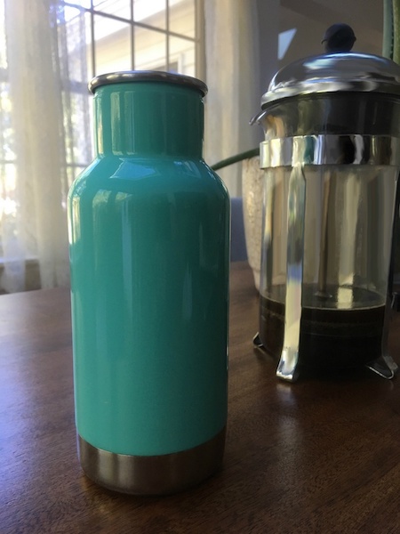
Before we do anything else, let’s pour some 90°C coffee into a vacuum flask and consider the material properties of the model.
Materials involved:
- The coffee is represented using material properties of water
- The screw topper and insulation ring are both made of nylon
- The flask is made up of two stainless steel walls with a plastic foam filler in between (the inner gap in vacuum flasks is usually filled with evacuated air, but it may also contain foam)
All material properties except for the foam filler can be pulled directly from the Material Library in the COMSOL Multiphysics® software. As always, when using COMSOL Multiphysics, you can add special material properties manually into the software. In the case of the foam in this example, you would enter the following values:
- Conductivity: 0.03 W/(m·K)
- Density: 60 kg/m3
- Heat capacity: 200 J/(kg·K)
Tip: The modeling approaches mentioned here are both covered in the Natural Convection Cooling of a Vacuum Flask tutorial model. Please refer to the tutorial MPH file and accompanying documentation to see exactly how to set up and solve this model, because we won’t go into detail in this blog post.
The Quick Approach: Using Predefined Heat Transfer Coefficients
For a quick and simple model, you can describe the thermal dissipation using predefined heat transfer coefficients. This method should help us determine how the coffee cools over time inside the vacuum flask. It’s simple because it won’t tell us anything about the flow behavior of the air around the flask, and it’s useful because it will show us the cooling power over time.
Instead of computing heat transfer and flow velocity in the fluid domain, you would simply model the heat flux on the external boundary of the vacuum flask, defined from the heat transfer coefficient, the surface temperature, and the ambient temperature (25°C; a little warmer than standard room temperature):
q = h(T∞-T)
There are many predefined cases where h is known with high accuracy. The Heat Transfer Module (an add-on to COMSOL Multiphysics) includes a library of heat transfer coefficients for easy access.
Another time-saver with this method is the fact that you can avoid predicting whether the flow is turbulent or laminar, because many correlations are valid for a wide range of flow regimes. As long as you use the appropriate h correlations, you can typically arrive at accurate results at a very low computational cost with this method.
What about the second approach? It’s worth considering how the cooling power is distributed on the flask surface as the coffee cools down. To do so, you need to include surrounding fluid flow in the model.
The Detailed Approach: Computing the Convective Velocity Field
To get a more complete picture of what’s going on with our precious java (seriously, when can I drink it?), we could create a more detailed model of the convective airflow outside the vacuum flask.
Taking the second approach calls for using the Gravity feature available in the Single-Phase Flow interface with the Heat Transfer Module or the CFD Module, which allows you to include buoyancy forces in the model. Typically, you would first need to figure out whether the flow is laminar or turbulent before following this modeling approach. For the sake of brevity here, let’s skip ahead: we know from the tutorial model documentation that the flow is laminar in this case.
The detailed model shows that the warm flask drives vertical air currents along its walls. The currents eventually combine in a thermal plume above the flask and air in the surrounding area is pulled toward the flask, feeding into the vertical flow. (This flow is weak enough that there are no significant changes in dynamic pressure.)
The vortex that forms above the flask’s lid reduces the cooling in that region — something you can’t tell from the first method. In essence, the fluid flow model is better at describing local cooling power than the simple method with the approximated heat transfer coefficient.
Comparing (and Combining) the Two Approaches
So how long will the coffee stay warm in the vacuum flask? Many coffee drinkers like to stay within the range of 50–60°C (roughly 120–140°F), because it’s supposedly when the “coffee notes shine.” Both methods suggest that after 10 hours inside the flask, the coffee will be about 54°C, which is still within the enjoyable range. Of course, if we were to bring the flask outside in cooler temperatures than the assumed 25°C, the coffee would cool down quicker.
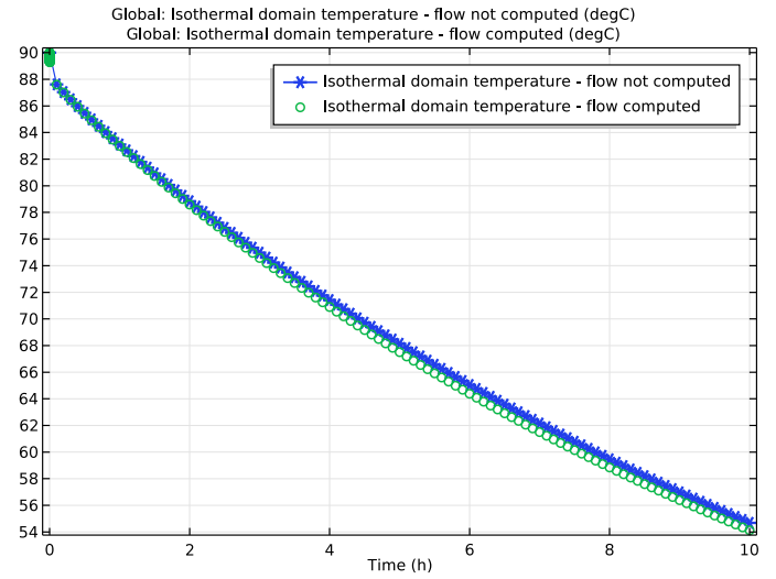
A plot of the coffee temperature over time for the two modeling approaches. The blue line denotes the first approach and the green line denotes the second approach.
Though both modeling approaches give very similar results in terms of the coffee temperature over time, it’s a different story when looking at the flask surface’s cooling power:
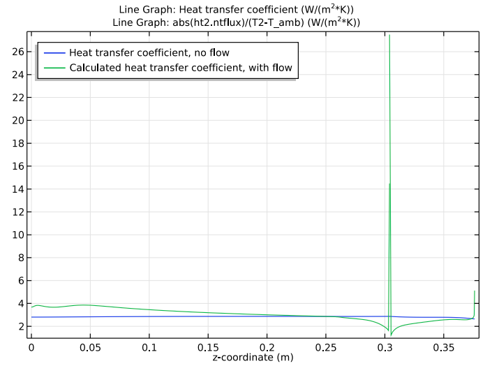
A plot of the heat transfer coefficient for the two modeling approaches. The blue line denotes the first approach and the green line denotes the second approach.
For fast and accurate results in the long run, you can combine the two approaches. After setting up the more detailed model, you can create and calibrate functions for heat transfer coefficients to use later, via the simpler approach for solving large-scale and time-dependent models.
Next Step: Try It Yourself
We saw that there are two different ways to model the convective cooling of coffee inside a vacuum flask over time. The detailed approach is more computationally demanding, as it combines heat transfer and fluid flow, but it’s also more accurate in the sense that it accounts for local effects. By combining both methods, you can save time in the future.
Try it yourself by downloading the tutorial model from the online Application Gallery or within the Application Library inside the COMSOL Multiphysics software. If you have any questions about this model or the COMSOL Multiphysics software, please contact us.


Comments (3)
BABU BIKASH GOGOI
January 23, 2018Hello madam,
I liked your blog. I am very new to this software. I am interested to discuss with you regarding the modelling of dispersed flow for a fluidised bed. If you are expert in that field, can you please help me with that?
Thanks in advanced!
Fanny Griesmer
January 24, 2018 COMSOL EmployeeHello there,
Thank you for your kind note. Depending on what type of assistance you need, I would recommend one of these options:
Athena Serra
August 7, 2018Bonjour,
je m’intéresse en ce moment au logiciel Comsol pour valider mon travail de recherche.
j’ai une cavité en forme de triangle (cône) en coordonnées cylindriques. Convection naturelle, les équations sont écrites sous forme de fonction de courant- vorticité + l’équation de l’énergie (Température) . Tout cela sans dimension. les conditions aux limites sont de type Rayleigh-Bénard.