Attitude detection, the measurement of an object’s orientation and rotation in three-dimensional space, is a crucial element in aircraft and spacecraft navigation. Recently, ring laser gyroscopes and fiber ring gyroscopes have proven to be viable alternatives to traditional mechanical gyros for accurately measuring rotations. The fundamental operating principle of such devices is an optical phenomenon called the Sagnac effect. In this blog post, we’ll employ ray optics simulation to observe this effect in a basic Sagnac interferometer.
Is It Just Me or Is the Room Spinning?
One of the basic tasks of any navigation system is to keep track of an object’s position and orientation, as well as their rates of change. Extreme accuracy may be required, particularly in space travel. For example, a communications satellite can be sensitive to angular velocities as small as one thousandth of a degree per hour.
While this accuracy requirement may seem daunting, this fundamental task of attitude control can be posed as a simple question: How do I determine how fast I’m spinning, and about what axis?
In principle, this task is the same for any observer in any rotating frame of reference — even a guest in the revolving restaurant shown below.
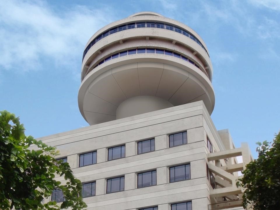
A photograph of the revolving restaurant at Ambassador Hotel, the oldest revolving restaurant in India. Image by AryaSnow — Own work. Licensed under CC BY-SA 4.0, via Wikimedia Commons.
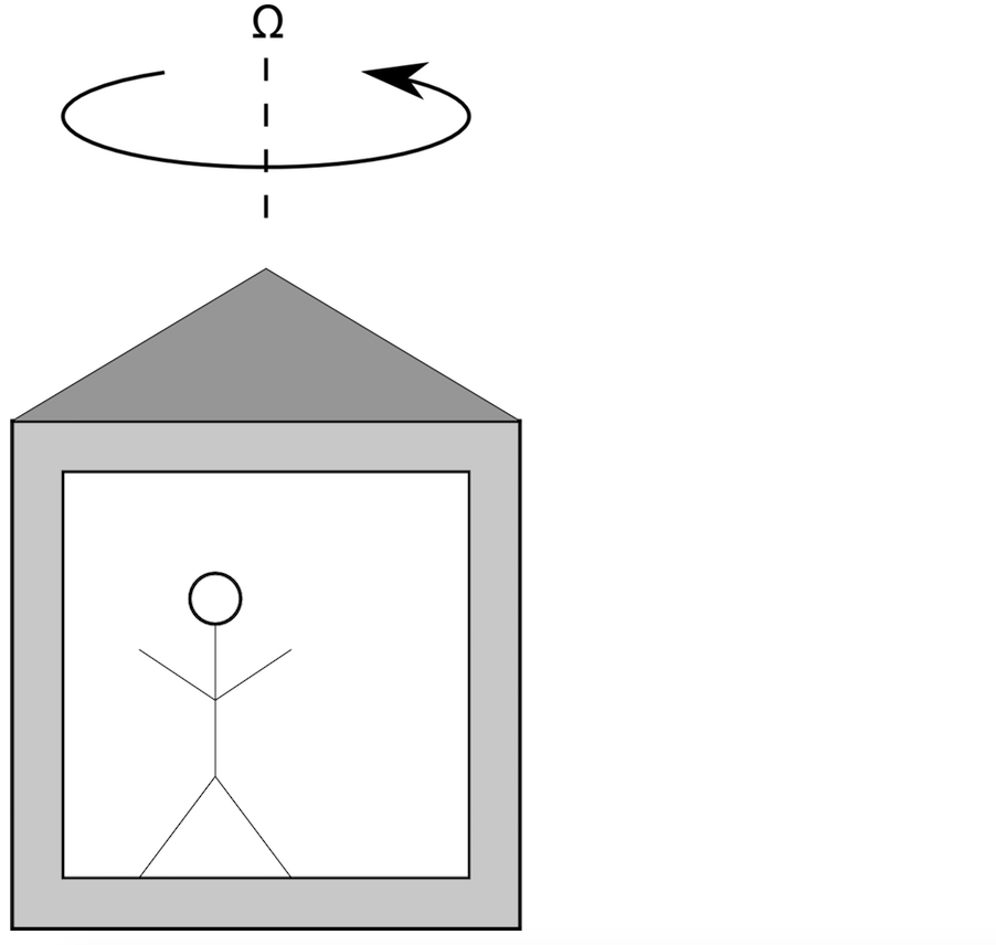
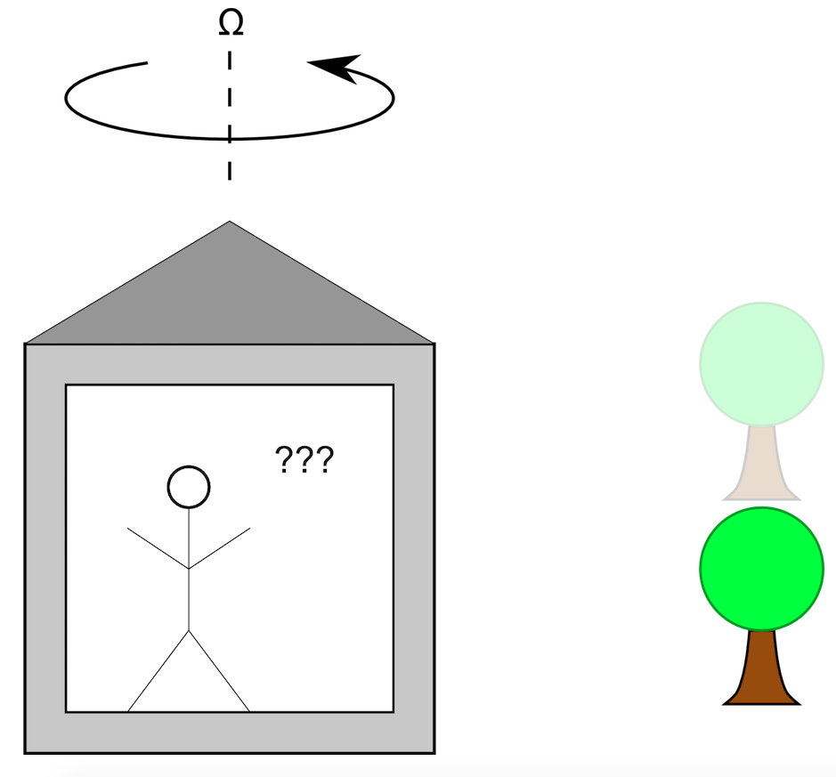
Suppose you’re the guest in such a rotating restaurant, trying to determine its angular velocity, Ω (unit: rad/s).
The simplest approach is to look outside. Pick a stationary object, like a building or a tree, and see if its location is changing over time in your field of view.
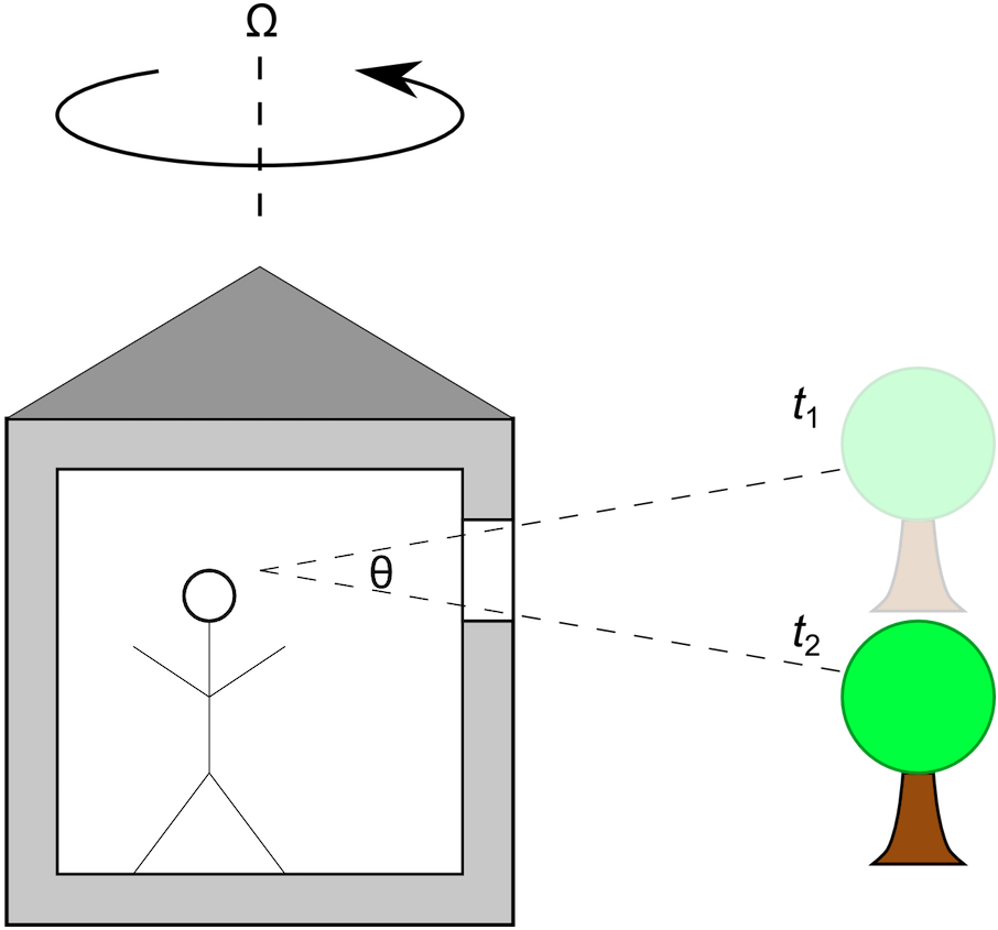
The above image shows the position of a tree in the observer’s field of view (i.e., through the window) at an initial time t1 and a later time t2. Let θ (unit: rad) be the angle between these two lines of sight. If the tree is very far away compared to the size of the restaurant, you could estimate the angular velocity as
A Similar Situation in Space
Because space travel is so much more demanding than the restaurant example described above, there are a few caveats to consider. In space, the idea of a “stationary object” is a bit tricky. For example, when using a Sun sensor for attitude control of a satellite in a geostationary orbit, you must also account for the relative motion as Earth orbits around the Sun. A star sensor, on the other hand, can be extremely accurate because stars other than the Sun can be considered fixed in space for many purposes, and because a star more closely approximates a point of light rather than a continuous source over some finite angle.
Because of the accuracy requirements of spacecraft attitude detection and control, the finite size of the object being observed must also be considered. For a line of sight to the Sun, for example, you need to know what part of the Sun you’re looking at. For arbitrary rotation in 3D, at least two objects are needed, because you don’t always know how the axis of rotation is oriented.
Obstructing the Field of View
Next, suppose we’re back at the restaurant, except that all of the windows are covered. Because your view of the outdoors is blocked, you can’t rely on any stationary object to get information about your rotating frame of reference.
There are several experiments you could perform within your rotating frame of reference to determine its angular velocity. For example, you could put a ball on the floor and see if it rolls, presumably due to a centrifugal force. (This requires that you know where the axis of rotation is — not always a given in space travel!) Another approach would be to use a mechanical gyroscope.
A third approach, explained in the following section, is to exploit the unique properties of light; namely, its uniform speed in a vacuum in all frames of reference. When light propagates in a rotating frame of reference, it reveals a phenomenon known as the Sagnac effect. A ring laser gyroscope takes advantage of this effect. Such gyroscopes have become a popular alternative to traditional mechanical gyroscopes, which use rotating masses, because the ring laser gyro has no moving parts, thus reducing the cost of maintenance.
Explaining the Sagnac Effect
The easiest way to visualize the Sagnac effect is to consider two counterpropagating light rays — that is, two rays going in opposite directions — that are constrained to move in a ring. The ring is rotating counterclockwise with a constant angular velocity Ω. (The SI unit is radians per second, but for inertial navigation systems, we might work in degrees per hour instead.)
The two rays are initially released at a point P0 along the ring. The rays go around the ring at the speed of light in opposite directions, while the release point rotates with the frame of reference. By the time the clockwise ray returns to the release position, it has moved to a new location shown by P1, and the distance it has traveled is somewhat less than one full circle. By the time the counterclockwise ray returns to the release position, it has moved to a different location, P2, and the distance it has traveled is greater than one full circle.
Of course, the movement shown here is greatly exaggerated. In reality, the displacement of P1 and P2 from P0 (and from each other) might be 10 billion times smaller! Even then, the tiny difference in the distance traveled (and similarly, the transit time) between the two rays is detectable because it’s accompanied by a phase shift, which produces an interference pattern between the rays. If we let ΔL represent the difference in the distance traveled by the two rays, then
(1)
where A is the area of the ring and c0 = 299,792,458 m/s is the speed of light in a vacuum.
As it turns out, Eq. (1) isn’t just true for circular paths, but for other shapes as well. The optical path difference only depends on the area enclosed by the loop and not by its shape. A more general derivation of Eq. (1) can be accomplished using the principles of general relativity. At its core, the Sagnac effect is a relativistic phenomenon, for which a classical derivation gives the same results to first order. For a more rigorous application of the theory, see Refs. 1–2.
Demonstrating the Sagnac Effect with Ray Optics Simulation
In this section, we examine a model of a basic Sagnac interferometer. This shares the same fundamental operating principle as the ring laser gyro, but is simpler to set up because we don’t need to consider the presence of a lasing medium along the beam path. (Besides the intensity gain, such a lasing medium can introduce many other complications, such as dispersive effects, that we can ignore for illustrative purposes.) However, a Sagnac interferometer with a given geometry will introduce the same optical path difference and phase delay as a ring laser gyro with the same arrangement of mirrors, so we can still learn quite a lot from it.
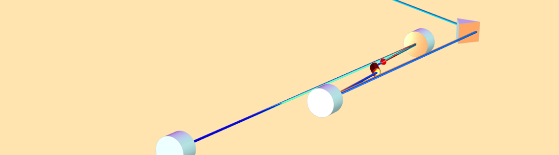
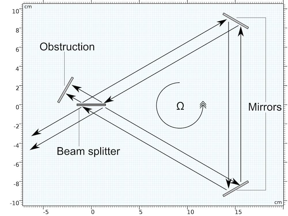
The basic Sagnac interferometer geometry consists of a beam splitter, two mirrors, and an obstruction to absorb the outgoing rays. It is illustrated below.
A few geometry parameters for this model are tabulated below.
| Name | Expression | Value | Description |
|---|---|---|---|
| λ0 | N/A | 632.8 nm | Vacuum wavelength |
| R | N/A | 10 cm | Ring radius |
| b | b=R\sqrt{3} | 17.3 cm | Triangle side length |
| P | P = 3b | 52.0 cm | Triangle perimeter |
| A | A = b^2 \sqrt{3}/4 | 130 cm2 | Triangle area |
The geometry is sometimes designed in a square rather than a triangle, with mirrors at three vertices and a beam splitter at the other. Rays are traced through the system with directions indicated by arrows. Because the whole apparatus is rotating counterclockwise, the rays going counterclockwise propagate a slightly longer distance than the rays going clockwise, before reaching the obstruction.
To better visualize this phenomenon, see the two animations below. (Note again that the rotation here is exaggerated by a factor of about ten billion!)
In the left animation, the observer stands in an inertial (nonaccelerating) frame of reference. Thus the rays go along straight paths but they hit the mirrors at different times. In the right animation, the observer is “riding” the spacecraft and is thus in a noninertial frame. (Strictly speaking, even in this rotating frame, the counterpropagating rays go at the same speed; the speed of light is the same in any frame of reference!)
For the geometry parameters given above, applying Eq. (1) gives the optical path difference between the counterpropagating rays as about 8 × 10-16, or 0.8 femtometers. This is about the radius of a proton; clearly a difficult quantity to measure! Rather than report path length directly, Sagnac interferometers and ring laser gyros usually report the frequency difference or beat frequency Δν, given by
(2)
where ν (in Hz) is the frequency of the light, and L is the optical path length for light going around the perimeter of the triangle.
Note that L is not necessarily the perimeter of the triangle itself, since there might be a comoving medium such as a lasing medium with n ≠ 1 along the beam path. In this example, we assume the space between the mirrors and beam splitter is a vacuum. The beat frequency is on the order of 1 Hz, which is certainly much easier to measure than a distance equal to the proton radius.
This model uses the Geometrical Optics interface to trace rays through the Sagnac interferometer geometry. The two mirrors are given the dedicated Mirror boundary condition, which causes specular reflection. The beam splitter uses the Material Discontinuity boundary condition with a user-defined reflectance of 0.5, so that both of the counterpropagating beams have the same intensity.
To rotate the apparatus, use the Rotating Domain feature, as shown below.

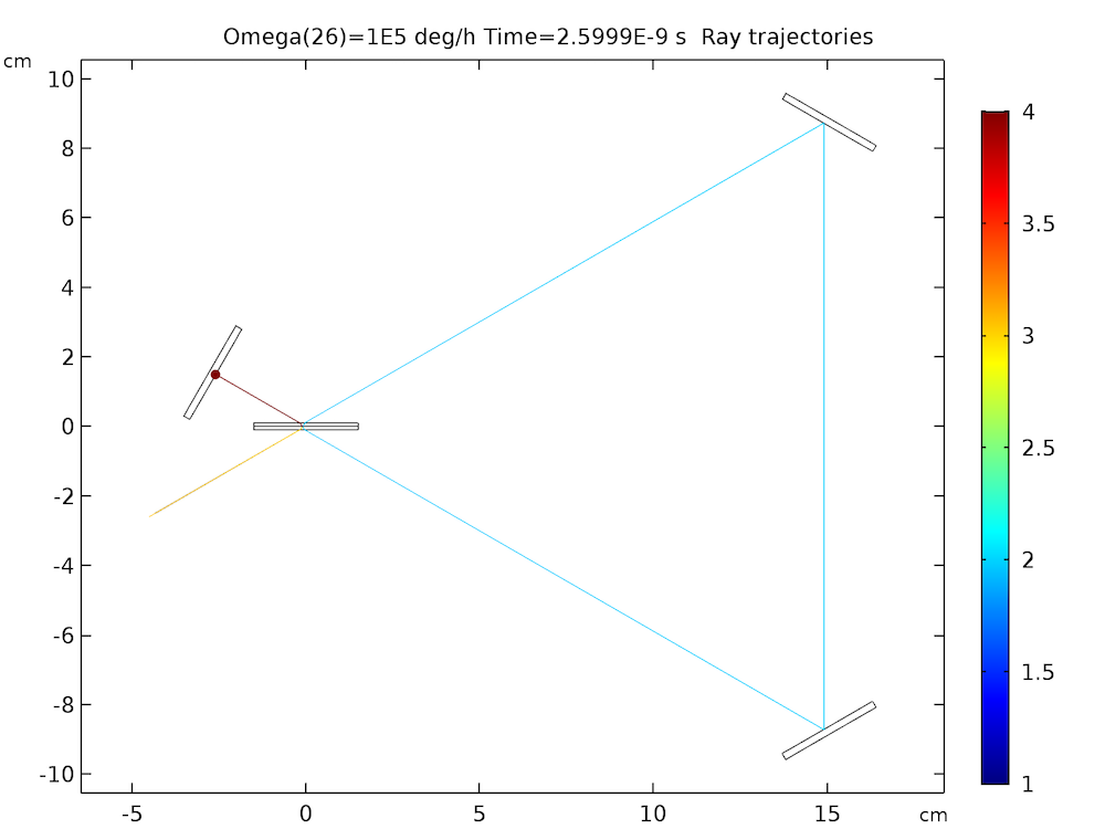
The resulting plot shows the rays propagating in both directions through the system of mirrors, but because the mirrors move so slowly relative to the speed of light, the two paths are indistinguishable in this image. If we zoomed in by a factor of 10 billion or so, we’d be able to discern two triangles spaced a tiny distance apart.
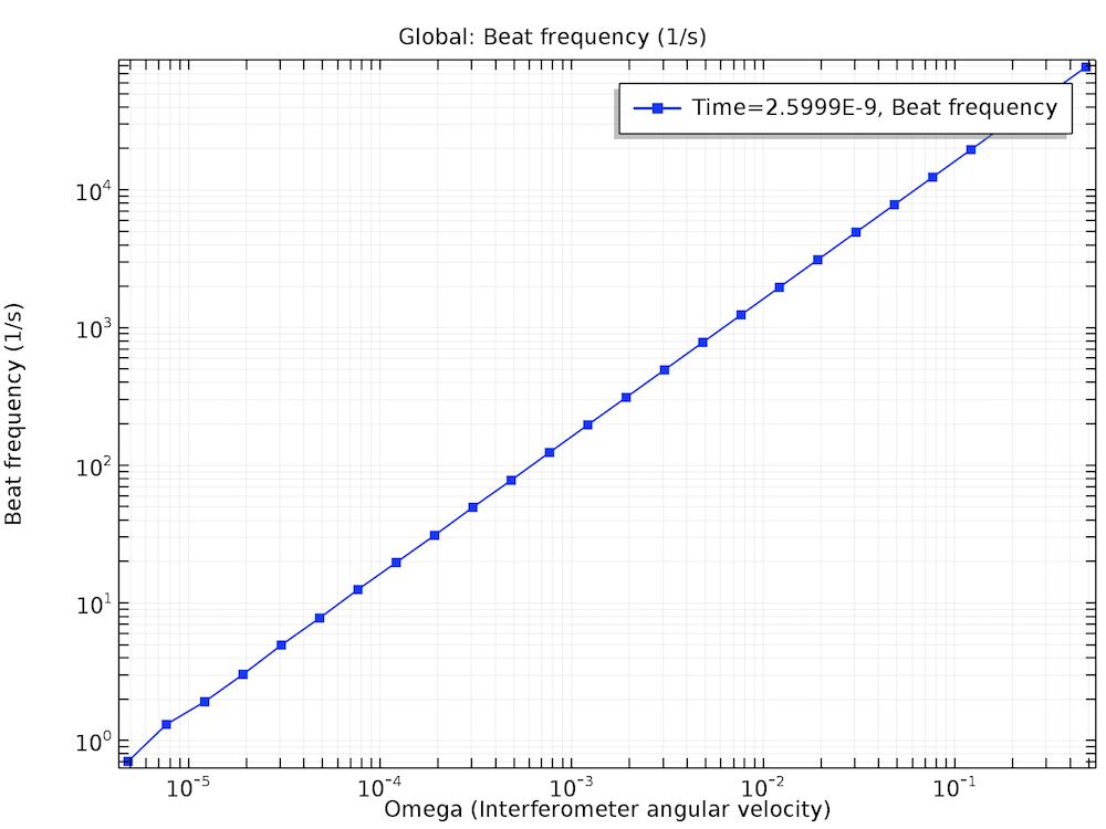
In the following plot, the beat frequency is given as a function of the angular velocity of the interferometer. As expected from Eqs. (1)–(2), this relationship is linear. Some numerical noise is visible in the bottom-left corner of the plot. This is due to numerical precision and is explained in greater detail in the model documentation.
Applying Attitude Detection to Aircraft and Spacecraft Navigation
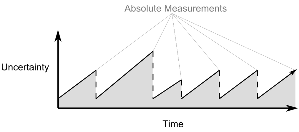
The Sagnac interferometer described above, along with related devices like ring laser gyros and fiber optic gyros, are examples of inertial navigation systems, which predict an object’s position and orientation by starting from a known position and then integrating the translational and angular velocity over time. In practice, inertial navigation systems are usually combined with absolute measurements of position and orientation relative to some other object in space. This absolute measurement might be done with an Earth sensor, Sun sensor, or star sensor; with RF beacons at known locations on the earth’s surface; with measurements of the earth’s magnetic field; or with any combination of these.
The uncertainty of an inertial navigation system grows over time due to small errors in the measurement of the translational and angular velocity. Periodically taking an absolute measurement using one of the sensors described above resets this uncertainty to a more reasonable value. A prediction of the uncertainty over time might look like the following graph.
Conclusions
We’ve successfully demonstrated the Sagnac effect in a simple interferometer using ray optics simulation. The resulting beat frequency agrees with the more rigorous theory, which is based on general relativity, as long as the velocity of all of the moving parts is much smaller than the speed of light. The magnitude of the optical path difference due in a Sagnac interferometer or ring laser gyro depends only on the area enclosed by the counterpropagating beams, not on the geometry of the loop.
Next Step
Explore the Sagnac interferometer model by clicking the button below.
References
- Post, Evert J. “Sagnac effect”, Reviews of Modern Physics, 39, no. 2, p. 475, 1967.
- Chow, W.W. et al. “The ring laser gyro”, Reviews of Modern Physics, 57, no. 1, p. 61, 1985.


Comments (1)
Jeffrey Wagner
July 3, 2018Great paper !