
In the first part of this blog series, we discussed variational problems and demonstrated how to solve them using the COMSOL Multiphysics® software. In that case, we used simple built-in boundary conditions. Today, we will discuss more general boundary conditions and constraints. We will also show how to implement these boundary conditions and constraints in the COMSOL® software using the same variational problem from Part 1: (the soap film) — and just as much math.
Classifying Constraints
There are several schemes of classifying constraints. Here, we will consider those that have the most implications for computational implementation.
Based on the geometric entity concerned, we can have point (isolated), distributed, and global constraints. For example, on one hand, the boundary conditions in a 1D problem are constraints at isolated points. On the other hand, a condition that should hold at every point is a distributed constraint. Global constraints specify some norm (usually an integral) of the solution. For example, specifying the length of a catenary cable or surface area of a soap film provides a global constraint.
Some people use the term pointwise constraint for a distributed constraint. We would like to make a clear distinction between that and what we are calling a point constraint here. A point constraint is enforced at a single point or a finite number of isolated points. This set of points has no length, area, or volume. Distributed constraints, however, hold at every point of a region. This can be every point of an edge, surface, or domain of a 3D object.
Another classification is equality constraints versus inequality constraints. A familiar inequality constraint in structural mechanics arises in contact mechanics. The gap between contacting objects in an assembly has to be nonnegative. In chemical reaction engineering, lower bounds on species concentrations are also inequalities.
These classifications overlap. For instance, we can have distributed inequality constraints and distributed equality constraints and so on. Inequality constraints are mathematically more challenging, so we will focus on equality constraints first and move on to the former a bit later in the series.
Brief Introduction to the Theory of Equality Constraints
The calculus problem
is solved by finding the stationary points of the augmented objective function
with respect to both the coordinate \bf{x} and the Lagrange multiplier \lambda.
This same idea is used, albeit with appropriate extensions, in variational calculus. Consider the problem
Here, the distributed constraint g(x,u,u^{\prime})=0 has to be satisfied at all points in our domain and not just at one point. Thus, each point will have its own Lagrange multiplier, making \lambda a function and not just one number. Accordingly, the augmented functional is
(1)
Having turned the constrained variational problem for one field, u(x), to an unconstrained problem in two fields, u(x) and \lambda(x), we turn our attention to the optimality criteria. It is important to note here that we can make independent variation in both the solution field and the Lagrange multiplier field. That gives us the first-order optimality criteria
\frac{d}{d\epsilon_2}E[u+\epsilon_1 \hat u,\lambda+\epsilon_2 \hat{\lambda}]\bigg|_{(\epsilon_1=0,\epsilon_2=0)} = 0.
In terms of F and g, we have
These are the equations we need to enter in the Weak Form PDE interface. We will quickly return to that. First, let’s derive the corresponding conditions for global (integral) and point (isolated) constraints.
When we have a global constraint
the augmented functional is
where \lambda is one number and not a field.
The first-order optimality conditions are
Finally, using the properties of the Dirac delta function, the point (isolated) constraint g(x,u,u^{\prime})=0, \textrm{ at } x=x_o can be thought of as the global constraint
Dirac delta functions can be analogously utilized to derive constraints on edges in 2D and 3D, and surfaces in 3D.
Plugging the above result in the formulation for global constraints, we get the first-order optimality conditions
(2)
(3)
If we have more than one isolated point constraint, we will have a Lagrange multiplier for each point. The Lagrange multiplier will not be a field, but a finite set of scalars, one valid at each isolated point. If we have a distributed constraint that is not imposed on the whole domain but over parts of a domain, we can define the Lagrange multiplier only over that part. Here, we will have a Lagrange multiplier field.
Implementing Constraints in COMSOL Multiphysics®
Let us now see how to implement constraints in COMSOL Multiphysics. We will consider the same soap film problem from the previous blog post, but with the following boundary conditions.
The first boundary condition is something we could have specified using the Dirichlet Boundary Condition node, but for pedagogic reasons, we will use the more general constraint framework. The two boundary conditions above can be rewritten as
We need the partial derivatives of the constraint equations with respect to u and u^{\prime}.
Finally, we will plug these as weak contributions at the corresponding points. The contribution from F remains the same as before.
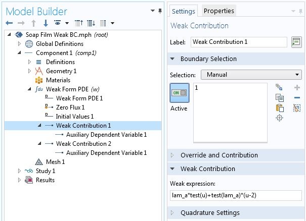
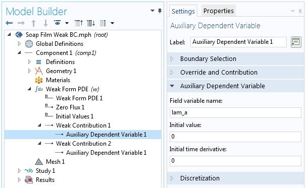
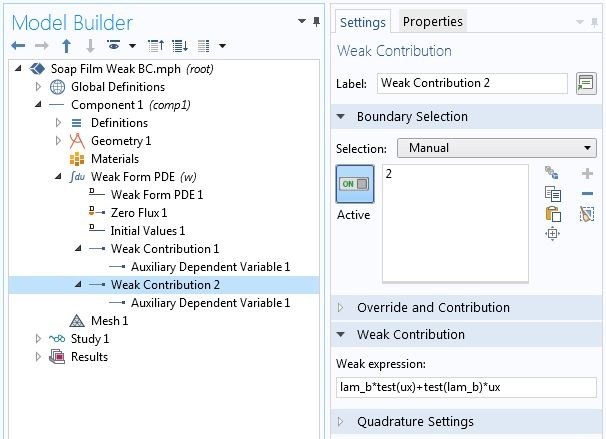
Specifying point constraints using point weak contributions.
Note that the point contribution from (Eq. 3) and the second term in (Eq. 2) have been added together in the Weak Contribution 1. The logic here is that, since \hat{u} and \hat{\lambda}_a are independent variations, setting the sum of terms containing those variations to zero is equivalent to setting terms containing each variation to zero. The numerical solution for this variational problem with the above constraints is shown in the plot below.
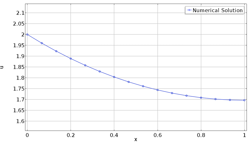
Solution with radius 2 at the left end and zero slope at the right end.
In the theory section, we discussed different types of constraints. The table below summarizes the recommended places in the software where contributions from constraints are specified and unknowns (Lagrange multipliers) are defined based on the type of constraint.
|
Constraint Type |
Examples | Constraint Contribution Containing \hat{u} | Constraint Contribution Containing \hat{\lambda} | Where to Define \lambda |
|---|---|---|---|---|
| Distributed constraint |
|
Weak contribution | Weak contribution |
|
| Global (integral) constraint |
|
Weak contribution | Global Equations node | Global Equations node |
| Isolated point constraint |
|
Weak contribution | Weak contribution |
|
Specifying Fluxes (Forces)
So far, we discussed specifying constraints. To this end, we introduced unknown Lagrange multipliers. In many physical problems, Lagrange multipliers are reaction forces or fluxes necessary to enforce a constraint. If instead of the constraint, you know the applied forces or fluxes, how do you specify that?
Go back to the functional to be minimized and reformulate, including the forces (fluxes). For example, for boundary loads in structural mechanics, this adds the virtual work due to the loads. The expression to enter in the COMSOL Multiphysics interface is similar to what we had to do for constraints. The known value of the force (flux) goes in place of the Lagrange multiplier, and we do not need auxiliary variables for Lagrange multipliers. As a result, the term containing the variation of the Lagrange multiplier disappears.
Find more information in our previous blog post on how to add point loads (sources) using weak contributions.
Adding Constraints to Points That Are Not in the Geometry Sequence
Occasionally, we want to add a constraint to a point in our domain that is not explicitly inserted (or created by intersection of curves) in the geometry sequence. We cannot select the point and associate it with the point weak contribution as shown in the above example. However, we can add a global weak contribution and use a domain point probe to refer to the solution and its variation.
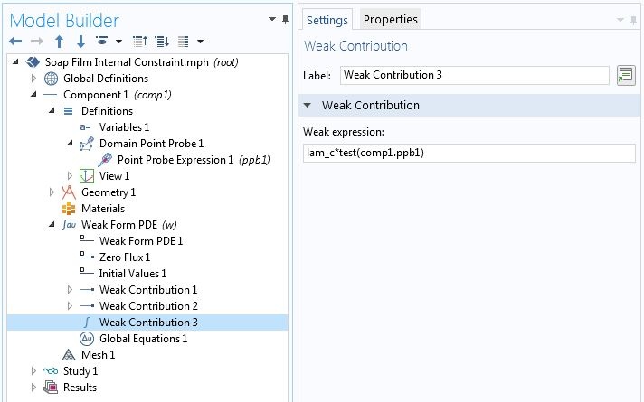
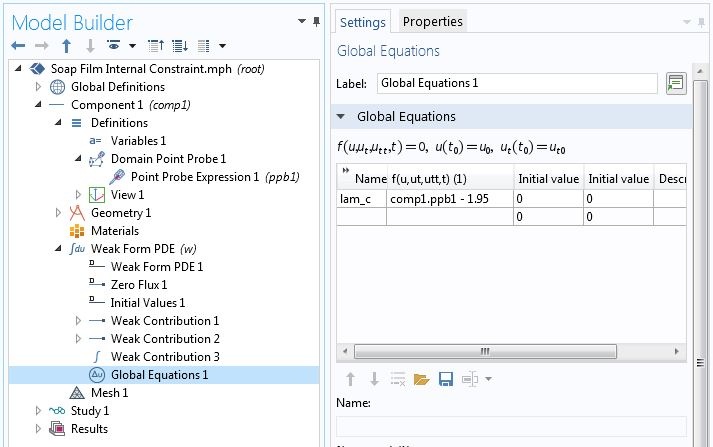
Consider a catenary cable supported at two ends. For a cable with uniform weight per unit length the variational problem is the same as the axisymmetric soap film problem. Thus, we will use the same COMSOL model. Additionally, we want to constrain the height u to 1.95 at the center without adding a point node to the geometry sequence. First, we add a domain point probe for u. Let the name of the probe be ppb1. The weak contribution corresponding to (Eq. 1) is lam_c*test(comp1.ppb1), where lam_c is a new Lagrange multiplier. We enter this contribution in the global Weak Contribution node as shown in the screenshot below. This node does not allow the creation of auxiliary variables, as opposed to weak contributions on explicitly defined geometric entities. However, we can add a Global Equation node where we can define the Lagrange multiplier and specify the constraint.
Adding a constraint on a point not in the geometry.
The plots below show the solution including that constraint. Circles are added at mesh nodes. The plot on the left shows the case where the central point does not have a mesh node associated with it. As such, the constraint is satisfied only approximately. On the right, we see the case of a solution on a finer mesh, where the mesher added a node where we want to impose a constraint. Here, the constraint is satisfied exactly.


Verifying internal constraints on points not in the geometry sequence. Aspect ratio is not preserved in plots.
A similar strategy can be used to add point loads (sources) for problems such as structural mechanics, heat transfer, or chemical transport. As mentioned earlier, such loads mathematically correspond to Lagrange multipliers. If we know the Lagrange multiplier, we do not add the Global Equation. Rather, we just have the weak contribution and, in place of lam_c above, we type the applied mechanical, thermal, chemical, or other type of load.
Stay Tuned!
So far in this blog series, we have shown how to solve variational problems using the Weak Form PDE interface and how to include equality constraints.
Constraints introduce additional complexity in the numerical solution. Mainly, they lead to saddle point problems, and a Lagrange multiplier implementation destroys the positive definiteness of the stiffness matrix. For nonlinear constraints, there is the additional danger of singular matrices during the nonlinear iteration. This can be especially problematic in global and distributed constraints.
In the next installment of this series, we will show numerical strategies for circumventing these issues. After we discuss these strategies using equality constraints, we will proceed to inequality constraints later in the series.


Comments (4)
Musa Aliyu
September 10, 2018Great work!
Mohammad Kazemi
April 12, 2020Thanks. What if the (distributed) constraint involves two different boundaries (similar to periodic boundary conditions)? How can one enforce that?
James Z
January 30, 2023Dear Kindo:
Thanks for this blog. It’s very useful for us to understand the weak contribution. I have some doubts about this sentence ‘the point contribution from (Eq. 3) and the second term in (Eq. 2) have been added together in the Weak Contribution 1’. As we can see from the picture, the weak contribution was wrote in Comsol as ‘lam_a*test(u)+test(lam_a)*(u-2)’. ‘test(lam_a)*(u-2)’ is equation 3, ‘lam_a*test(u)’ is the right part of equation 2, so the question comes out. Where is the left part of equation 2 which is relating to F? Is it equals to 0, so it is not wrote in Comsol? It would be grateful if you help me with this. Thanks!
Xiaoyu Liang
October 14, 2023It’s unsolved in the third example refer to adding a point not in the Geometry sequence!