
What do soap films, catenary cables, and light beams have in common? They behave in ways that minimize certain quantities. Such problems are prevalent in science and engineering fields such as biology, economics, elasticity theory, material science, and image processing. You can simulate many such problems using the built-in physics interfaces in the COMSOL Multiphysics® software, but in this blog series, we will show you how to solve variational problems using the equation-based modeling features.
Minimizing Over Functions
In elementary calculus, we find optimal values for a function of single or multiple variables. We look for a single number or a finite set of numbers \mathbf{x} that minimize (maximize) a function f(\mathbf{x}). In variational calculus, we search for a function u(x) that minimizes (maximizes) a functional E[u(x)]. In some sense, we can think of this as infinite dimensional optimization. Roughly speaking, a functional takes a function and returns a number. For example, a definite integral is a functional.
In engineering problems, these functionals commonly represent some kind of energy. For example, in elasticity theory, we can find equilibrium solutions by minimizing the total potential energy. This terminology is often carried over to other variational problems, such as variational image processing. We call the functional the “energy” — even when it doesn’t physically represent energy in the usual sense.
A soap film between rings.
Consider a soap film between two rings on the yz-plane whose centers are on the x-axis. We want to find the function u(x) that gives us the shape of the soap film when we revolve the graph of the function around the x-axis. This function minimizes the following functional
(1)
More generally, in variational calculus, we are looking for a function u(x) that minimizes
(2)
Most engineering problems deal with functionals that contain, at most, a first-order derivative. In the beginning of this series, we will focus on such problems in one spatial dimension. Later on, we will generalize to higher dimensions, higher-order derivatives, and several unknowns. Lastly, maximizing is the same as minimizing the negative, thus we will only talk about minimization in the sequel.
The functional we will be dealing with, unless specified otherwise, is
(3)
Solving Variational Problems
Say you find yourself blindfolded in a valley. How do you know when you’ve reached the bottom? (By the way, removing the blindfolds is not an option.) You might feel the ground around you with your hands and feet, and if every area that you test feels higher than where you stand, you are at the bottom of the valley (at least on a local depression). The same idea is used to check minima in both calculus and variational calculus. In calculus, you test neighboring points, whereas in variational calculus, you test neighboring functions.
The function u(x) minimizes the functional E[u(x)] if and only if, for every admissible variation \hat{u}(x), it follows that
(4)
for a small number \epsilon.
Not every variation \hat{u} is admissible, since every u+\epsilon \hat{u} has to satisfy constraints on the solution. For example, for a soap film fixed to wires at the ends, every function we compare with the minimal function has to be fixed to the wires as well. Consequently, we only consider those variations with \hat{u}(a) = \hat{u}(b) = 0. We will deal with constraints in detail in later blog posts.
A necessary condition for Eq. 4 is
(5)
assuming sufficient smoothness to allow differentiation.
In this series, we are not going to discuss problems with moving or open boundaries. In such cases, we can move the derivative inside the integral and apply the chain rule to obtain
(6)
Note that we vary only the dependent variable u and its derivatives, not the spatial coordinate x.
If you are interested in problems with moving boundaries or interfaces, check out these blog posts on using the level set and phase field methods for free surface problems and modeling free surfaces with moving mesh.
As shown in Eq. 1 for soap films, we have F(x,u,u^{\prime}) = u\sqrt{1+u^{\prime}^2} \Rightarrow \frac{\partial F}{\partial u} = \sqrt{1+u^{\prime}^2}, \frac{\partial F}{\partial u^{\prime}} = \frac{uu^{\prime}}{\sqrt{1+u’^2}}. Consequently, the variational problem for soap films is to find u(x) such that
(7)
Euler-Lagrange Equation
In classical variational calculus, we apply integration by parts to move the spatial derivative from the variation \hat{u} to the solution u to obtain the Euler-Lagrange equation
(8)
and use ordinary differential equation (ODE) methods to find the solution.
In higher dimensions, the Euler-Lagrange equation becomes a partial differential equation (PDE).
In our case, we do not need to use the Euler-Lagrange equation, so we will not talk about it any further. The reason is that the finite element method works with the variational formulation. In COMSOL Multiphysics, for example, if you use the Coefficient Form PDE or General Form PDE interfaces to specify the Euler-Lagrange equation, the software internally formulates and solves the corresponding variational equation, so why waste the effort? As we will see later, the variational form also provides natural ways of thinking about sophisticated domain and boundary conditions.
Implementing a Variational Problem in COMSOL Multiphysics®
To specify a variational problem in COMSOL Multiphysics, we use the Weak Form PDE interface. How do we differentiate between the solution u and the corresponding test function \hat{u}? For the latter, we can use the test operator. For example, for the soap film problem, the integrand in the variational formulation has to be entered as sqrt(1+ux^2)*test(u) + u*ux/sqrt(1+ux^2)*test(ux) in the Weak Form PDE node, as shown below.
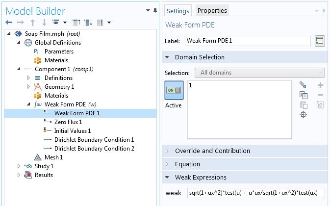
Specifying a variational problem.
We consider the simple constraint that the soap film is fixed on wire loops on the left and right sides. The radii of the left and right rings are 1 and 0.9, respectively, thus we know the primary variable u at both ends. The Dirichlet Boundary Condition node is used to specify such boundary conditions. For numerical reasons, in this particular problem, we provide an initial value of 1 instead of the default 0 in Initial Values 1.
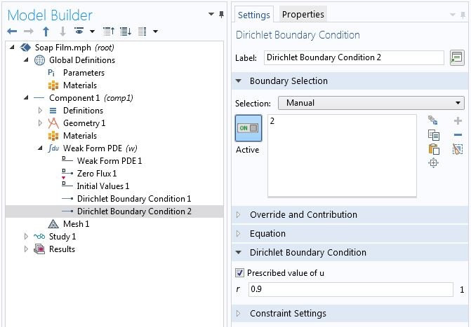
Using the Dirichlet Boundary Condition node to specify known boundary values.
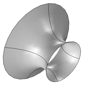
If we compute the solution, we obtain the shape shown below.
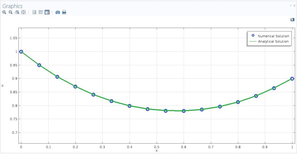
Profile of a soap film hanging between two vertical circular wire rings.
Specifying a Simpler Symbolic Problem
In the above example, we carried out the partial differentiation of F with respect to u and u^{\prime} manually. We can avoid unnecessary labor and potential errors by using the symbolic mathematics capabilities of COMSOL Multiphysics.


Using symbolic differentiation to reduce manual work.
Variational Solution Versus Direct Optimization
We can solve a functional minimization problem by direct optimization. In this approach, we do not need to derive the variational problem. On the downside, it requires more computational tools. In COMSOL Multiphysics, for example, direct optimization requires the Optimization Module. If you are interested in direct optimization, check out our blog post on solving the brachistochrone problem using the Optimization Module.
Coming Up Next…
Today, we showed you how to solve variational problems with simple constraints using the Weak Form PDE interface. This interface comes with every COMSOL Multiphysics installation. You can learn more about the weak form in this blog post.
In upcoming posts, we will show how to add more sophisticated constraints, such as point, distributed, and integral constraints. The series will conclude by generalizing to higher spatial dimensions, higher-order derivatives, and multiple fields. Stay tuned!
In the meantime, contact us to learn more about the equation-based modeling features of COMSOL Multiphysics via the button below.

Comments (2)
Mehrzad Tabatabaian
September 29, 2018is this model available, for download?
Thomas Gresham
January 22, 2019Hi Teme,
I have been going through this series and have found it to be very interesting! Variational calculus is such a fascinating topic, and this post did a great job of demonstrating the concepts in a relatable way.
I may have spotted a typo in equation 7. In the first term, is the u^2 meant to be a u’^2 as you have it written in the differentiation directly above equn 7? Same for one of the u in the numerator of the second term in equn 7?