

How do you find the shortest overland distance between two points across a lake? Such obstacles and bounds on solutions are often called inequality constraints. Requirements for nonnegativity of gaps between objects in contact mechanics, species concentrations in chemistry, and population in ecology are some examples of inequality constraints. Previously in this series, we discussed equality constraints on variational problems. Today, we will show you how to implement inequality constraints when using equation-based modeling in COMSOL Multiphysics®.
A Penalty Method for Path Planning
Assume you want to go from a point (0,0.2) to (1,1), but there is a circular obstacle centered at (0.5,0.5) and radius 0.2. The curve (x,u(x)) that minimizes the distance between two end points, (a,u(a)) and (b,u(b)), should minimize the functional
In the Euclidean space, the shortest distance between two points is a straight line. As such, solving for this equation using what we have discussed so far should give a straight line. However, in our case, that straight line goes through the obstacle. This is not feasible. We have to respect the constraint that our path cannot go into the obstacle; that is, the distance from a point on the path to the center of the circular obstacle should be greater than or equal to the radius of the circle.
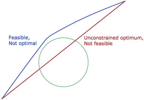
A basic schematic of the inequality constrained problem.
We want to add a term to our functional to penalize constraint violation. For an equality constraint g=0, we penalize both negative and positive values of g. For an inequality constraint g \leq 0, we have to penalize only positive values of g, while negative values are acceptable.
In the obstacle problem, this means we have to penalize only when the path tries to penetrate the obstacle. It is feasible, although maybe not optimal, to stray far from the shores of our circular lake, thus our penalty-regularized objective function is
where \mu is the penalty parameter and we used the ramp function
x& x\ge 0 \\
0 & x \le 0.
\end{cases}
For a general functional
to be minimized subject to the inequality constraint
the penalized functional becomes
The final step is to take the first variational derivative of the above functional and set it to zero. Here, we need to remember that the derivative of a ramp function is the Heaviside step function H.
In the above derivation, we used the fact that \big \langle x \big \rangle H(x) = xH(x). Note that we are discussing nonpositivity constraints here. Nonnegativity constraints can be dealt with by taking the negative of the constraint equation and solving for the equivalent nonpositivity constraint.
The first term in the above variational equation is the now-familiar contribution from the unconstrained problem. Let’s see how to add the penalty term using the Weak Contribution node. We will use the simpler Dirichlet Boundary Condition node to fix the ends.


Implementing an inequality constraint using the penalty method.
Note that in the above weak contribution, we did not include \frac{\partial g}{\partial u^{\prime}}, since the constraint in this problem depends only on the solution and not on its spatial derivative.
Solving this problem for a sequence of increasing penalty parameters, while reusing the previous solution as an initial estimate, we get the result shown below.
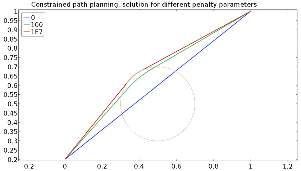
Finding the shortest path around an obstacle using the penalty method. A zero penalty returns the unconstrained solution.
In our discussion of the physical interpretation of the penalty method for equality constraints, we have said that the penalty term introduces a reaction proportional to the constraint violation. That interpretation applies, but for inequality constraints, the reaction is one-sided.
Imagine forcing a bead to stay in place using compressive springs. The springs are not hooked to the bead; they just touch. To keep the bead at x=0, we have to use two springs, one on each side of the origin. If it is acceptable for the bead to go to the left of the origin, our constraint is x \leq 0 and we have to place the compressive springs only on the right side. That is why we penalize \big \langle g \big \rangle instead of |g|.


A spring analogy of penalty enforcement of equality (multilateral) and inequality (unilateral) constraints.
The Lagrange Multiplier Method
When we discussed the numerical properties of different constraint enforcement strategies, we said that while the Lagrange multiplier method enforces constraints exactly, it has certain undesirable properties in numerical solutions. Namely, it is sensitive to initial estimates of the solution and can require a direct linear solver. These downsides are still there, but in inequality constraints, there is an additional challenge. Specifically, the constraint may not always be active.
Consider our path planning problem. In parts of the path not touching the obstacle, the constraint is not active. However, we do not know beforehand where the constraints will be active and not active. There are several strategies to deal with this, but we would like to point out two commonly used methods.
Active Set Strategy
Assume some constraints are active and some are not. In a distributed constraint, this means picking points where we expect g=0 and assuming the other points are inside the feasible region with g <0. At the inactive points, the Lagrange multiplier should be zero. On the active set, the Lagrange multiplier should not be negative. These are the so-called Karush-Kuhn-Tucker (KKT) conditions. If, after computation, the active set changes or the KKT conditions are violated, we have to appropriately update the active set and recompute. The following flowchart summarizes this procedure:
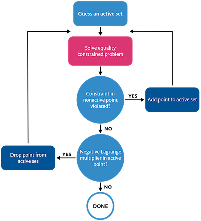
An active set strategy for the Lagrange multiplier enforcement of inequality constraints.
Through this iterative process, each iteration solves an equality constrained problem. Lagrange multiplier implementations of equality constraints have been discussed in the previous blog post in this series.
Slack Variables
Another strategy is introducing the so-called slack variables to change the inequality into equality. The constraint g \leq 0 is equivalent to g + s^2=0. Now we have an equality constraint involving a new slack variable. If the inequality is a distributed (pointwise) constraint, the slack variable as well as the Lagrange multiplier will be functions.
On one hand, the slack variable strategy introduces yet another unknown to be solved for, but solves the problem in one go. On the other hand, the active set strategy does not need this variable but has to solve multiple problems until the active set stops changing.
The Augmented Lagrangian Method
Like we did for equality constraints, let’s use a calculus problem to discuss the basic ideas of this method. Augmenting the unconstrained objective function with a Lagrange multiplier term with an estimated multiplier and a penalty term, we have
The first-order optimality condition for this constraint is
This suggests the multiplier update
If we start with a zero initial estimate for the Lagrange multiplier, the above equation updates the Lagrange multiplier only when g is positive. Thus, the Lagrange multiplier is never negative and is positive only on points that tend to violate the constraint.
The augmented Lagrangian method, being an approximate constraint enforcement strategy, will allow a small violation of the constraint. In fact, if there is no violation of the constraint, the Lagrange multiplier stays zero. As such, this strategy satisfies the dual feasibility part (\lambda \ge 0) of the KKT conditions exactly but satisfies the complementary slackness part (\lambda g = 0) only approximately. Both conditions are exactly satisfied with the Lagrange multiplier method.
Obstacles with Irregular Shapes
In today’s example, we used a very idealized lake whose boundaries could be described by a simple function. Or perhaps it was a pool. Sometimes, inequality constraints have such simple analytical forms. Nonnegativity constraints in chemical reactions or population dynamics are examples of this. However, other constraints do not have such simple forms.
For example, in contact mechanics, we want to keep the gap between contacting objects nonnegative, but the boundaries of the objects are rarely so simple that we can define them by smooth analytical functions. On top of that, for large deformation problems, we want to enforce the contact constraints on the deforming domains, but we definitely don’t have an analytical description of the deforming domains. As such, the constraints have to be satisfied on the discrete version of the objects obtained from the mesh. Complex search operations have to be used to find out, as the objects move and deform, what points come into and out of contact with other points. There are built-in features for this and other contact simulation procedures in the COMSOL Multiphysics® software.
For some simple geometries and deformations, we can conceivably use the General Extrusion operator to compute the distance between deforming objects without using the contact mechanics functionality. More complicated geometries would need the latter.
Up Next…
So far in this series, we have shown how to solve constrained and unconstrained variational problems using COMSOL Multiphysics and discussed the pros and cons of different numerical strategies for constraint enforcement. That said, we limited ourselves to 1D single-physics problems and variational problems with, at most, first-order derivatives in the functional.
With the basics of this subject covered, we hope we are ready to tackle higher dimensions, higher-order derivatives, and multiple fields. This will come in the next and final blog post in this series. Stay tuned!
View More Blog Posts in the Variational Problems and Constraints Series
- Part 1: Introduction to Modeling Soap Films and Other Variational Problems
- Part 2: Specifying Boundary Conditions and Constraints in Variational Problems
- Part 3: Methods for Dealing with Numerical Issues in Constraint Enforcement
- Part 5: Image Denoising and Other Multidimensional Variational Problems


Comments (2)
Yu Zhang
April 30, 2019Hi, Temesgen Kindo:
Thank you for providing this wonderful method to apply inequality constraint. Now I want to develop a damage model which involves the KKT condition, and need to calculate the Lagrangian multiplier. You mentioned the KKT condition in this blog. I am wondering whether it is possible to use your approach without programming to achieve that ?
Thank you for your help.
Regards,
Yu
William Huber
December 7, 2019Hello,
How was mu defined in he example here?
Thank you