

We previously discussed how to solve 1D variational problems with the COMSOL Multiphysics® software and implement complex domain and boundary conditions using a unified constraint enforcement framework. Here, we extend the discussion to multiple dimensions, higher-order derivatives, and multiple unknowns with what we hope will be an enjoyable example: variational image denoising. We conclude this blog series on variational problems with some recommendations for further study.
Variational Problems in Higher Spatial Dimensions
We have considered 1D problems and looked for a function u(x) that minimizes the functional
Now, let’s consider higher spatial dimensions while limiting ourselves to first-order derivatives. Consider the variational problem of minimizing
defined over a fixed domain \Omega.
For a neighboring function, u+\epsilon\hat{u}, this becomes
As with the 1D case, the necessary first-order optimality condition is
which means
To obtain variational derivatives, we have been forming a function that is essentially a function of the scalar parameter \epsilon and using single-variable calculus methods. A quicker formal way is to use the variational derivative notation as
for fixed domains.
Here, \delta u corresponds to \hat{u} in our previous notation. Notice that since the domain is fixed, we consider a variation of the function and its derivatives only. If the domain can vary with the solution, the variational derivative will have an extra contribution coming from the boundary variation.
Image Denoising: A Multidimensional Variational Problem
In recent decades, variational methods have yielded powerful and rigorous techniques for image processing, such as denoising, deblurring, inpainting, and segmentation. Today, we will use denoising as an example. One technique for image denoising is called total variation minimization. Say you have image data, u_o, that has been corrupted by noise. The image has speckles (sometimes called “salt-and-pepper noise”). You want to recover as much of the original image given by u as possible. As such, the image has to be denoised.
An image with erroneous details will have high variation; therefore, the denoised image should have as little variation as possible. A model after Tikhonov measures this total variation as
Minimizing just the total variation will aggressively smooth and return a solution close to a constant, losing legitimate details in the image. To prevent this issue, we also want to minimize the difference between the input data, u_o, and the solution, u, given by a fidelity term
Now that we have multiple, potentially conflicting objectives, let’s attempt a compromise by introducing the functional
where the regularization parameter \mu determines the emphasis on detail versus denoising (this is a user-specified positive number).
We are now ready to derive the first-order optimality condition, as discussed in the previous section. Requiring a vanishing variational derivative, we get
To demonstrate this process, we import an image into COMSOL Multiphysics and add a random noise to corrupt it. Here is what we get after ruining an image of a goose provided by my colleague:
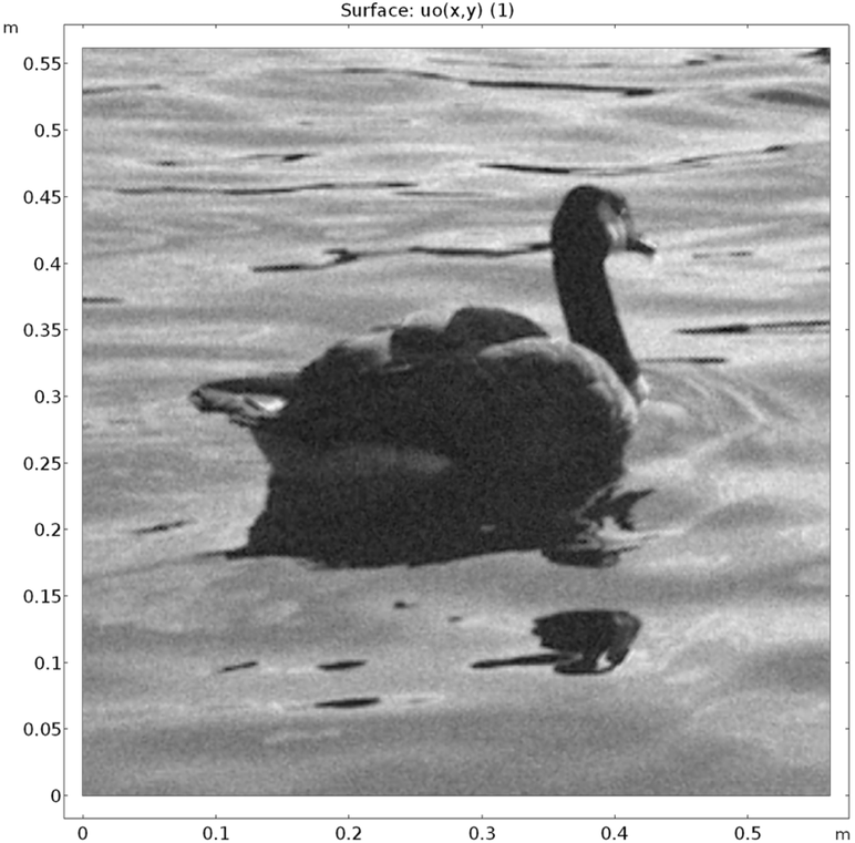
A test image deliberately corrupted by random noise.
The weak form above is given in vector notation. For use in computation, let’s write it out in Cartesian coordinates and leave out the common factor 2.
This can be entered into the COMSOL® software as shown in the screenshot below. We keep the data on the edge as is by using the Dirichlet boundary condition u=uo on all boundaries, and we use a regularization parameter of 1e6. In the simpler algorithms, the regularization parameter is determined by trial and error. We increase the parameter if the resulting image is missing relevant details and reduce it if the result is deemed too noisy.
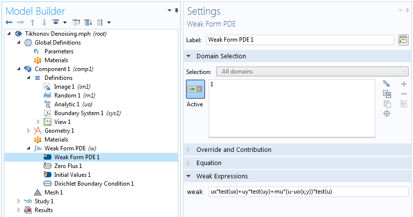
Specifying a variational problem in 2D.
Below is the denoised image, shown along with the original image — not bad for a rudimentary model!


Denoised image (left) and original image (right).
The Tikhonov regularization smooths too much and does not preserve geometric features such as edges and corners. The so-called ROF model with a functional given by
does better in this regard.
The first-order necessary condition for optimality, obtained by setting the variational derivative to zero, as done so far, is
Notice that the use of the absolute value in the functional results in a highly nonlinear problem. Also, the denominator |\nabla u| can go to zero in numerical iterations, giving a division-by-zero error. To prevent this, we can add a small positive number to it. In COMSOL Multiphysics, we often use the floating-point relative accuracy eps, which is about 2.2204 \times 10^{-16}.
The ROF model preserves edges but reportedly causes the so-called “staircasing effect”. Including higher-order derivatives in the functional helps avoid this.
Variational Problems with Higher-Order Derivatives
High-fidelity image processing and other subjects involve variational problems with high-order derivatives. A traditional subject in this respect is the analysis of elastic beams and plates. For example, in Euler beam theory, a beam with Young’s modulus E and cross-sectional moment of inertia I, loaded with lateral load f, bends to minimize the total potential energy
For small deformations, the analysis neglects the change of the domain, thus the variational formulation is to find u such that
Notice that we do not differentiate the Young’s modulus in the variational derivative because we are considering a linearly elastic material where material properties are independent of deformation. For nonlinear materials, the contribution to the variational derivative from material properties has to be included. This functionality is built into the Nonlinear Structural Materials Module, an add-on product to COMSOL Multiphysics.
The inclusion of higher-order derivatives in the functional does not introduce any conceptual change to the way we find the first-order optimality criteria, but it does have computational implications. Our finite element interpolation functions, picked in the Discretization section of the Weak Form PDE Settings window, need to have as much polynomial power, or higher, than the highest order spatial derivative in the variational form. For example, for the beam problem, there is a second-order derivative in the variational form, thus we cannot pick a linear shape function. If we did, all of the second derivatives in our equation would uniformly vanish. We have to use quadratic or higher-order shape functions.
Variational Problems with Multiple Unknowns
So far, we have considered minimizing functionals that depend on only one unknown, u. Often, the functionals contain more than one unknown. Say we have a second unknown, v, and a functional
The first variation of this functional is
Here, we assume the two fields, u and v, are independent of each other and, as such, we can take independent variations in both variables. Sometimes, this is not the case: There can be a constraint between the variables.
The easiest constraint between variables is when one is given explicitly in terms of the other, as in v = g(u). In such cases, we can opt to eliminate v from the problem by considering the functional
Generally, we have constraints of the form g(u,v,\dotsc)=0 and we cannot algebraically invert this expression. In such cases, we use the techniques considered in Part 3 of the blog series, which is about constraint enforcement. For example, for the Lagrange multiplier method, we have an augmented functional given by
where \lambda = \lambda(x,y,z) for a distributed constraint or
where \lambda is a constant for a global constraint.
We use the same Weak Form PDE interface to specify such multifield problems. The question is: Do we use a single interface or an interface for each unknown? It depends on the relationship between the unknowns. On one hand, if u and v are different components of the same physical vector, such as displacement or velocity, we can use the same interface and specify the number of dependent variables in the Dependent Variables section. On the other hand, if u represents temperature and v represents electric potential, we can employ different PDE interfaces. If, for some compelling reason, we have to use different discretizations or scales for different components of the same vector unknown, we can use multiple interfaces just as well. When we have multiple unknowns, we have to carefully choose the interpolation functions for each field (as discussed in a previous blog post on element orders in multiphysics models).
Concluding Remarks
Variational methods provide a unified framework to model a plethora of scientific problems. The Weak Form PDE interface, included in COMSOL Multiphysics, enables you to extend the functionality of the COMSOL® software by bringing in your own variational problems. In this series, we have demonstrated this power by solving problems that include finding the shape of soap films, planning paths for a hiker around a lake, and repairing corrupted images.
Bear in mind that several important partial differential equations do not come from minimizing a functional. The Navier-Stokes equation is one example. You can still use the Weak Form PDE interface to solve such problems after deriving their weak forms.
An important part of solving variational problems is specifying constraints. The previous three blog posts in this series deal with the mathematical formulation and numerical analysis of constraint enforcement.
A warning here is that we have only considered necessary conditions for optimality. Vanishing first-order derivatives are not sufficient for minima. First-order derivatives vanish on maxima as well. In the examples discussed in this series, we consider well-known problems where we know that the solution provides a minimum. When you are working on novel problems, make sure to check the second-order optimality criteria as well as the existence and uniqueness of the minimum (maximum) before cranking up the computation. For this and other more involved analytical and numerical aspects of variational problems, the following references are some of my personal favorites:
- A classic text on calculus of variations:
- I.M. Gelfand and S.V. Fomin (English translation by R.A. Silverman), Calculus of Variations, Dover Publications, Inc., 1963.
- More recent texts that discuss several engineering problems:
- K.W. Cassel, Variational Methods with Applications in Science and Engineering, Cambridge University Press, 2013.
- J.W. Brewer, Engineering Analysis in Applied Mechanics, Taylor & Francis, 2002.
- For constraint enforcement strategies:
- D.G. Luenberger, Introduction to Linear and Nonlinear Programming, Addison-Wesley Publishing Company, 1973.
- S.S. Rao, Engineering Optimization: Theory and Practice, John Wiley & Sons Inc., 2009.
Hopefully, this series has given you a taste of modeling variational problems using COMSOL Multiphysics, especially when what you want to model is not already built into the software.
Have fun, and feel free to contact us with any questions via the button below:

Comments (2)
Roberto Brambilla
September 25, 2018This series of posts on Variational Problems by Temesgen Kindo is fantastic!
Every COMSOL user ha to read them in order to better understand thw Weak Form and Weak Contribution. I hope he will continue to post more example and applications, also execises on these important arguments of Finte Element Method.
Temesgen Kindo
September 26, 2018Dear Roberto,
Thank you for the nice words!
We do have a blog post coming up on using weak contributions to add non-standard boundary conditions and constraints to physics interfaces.
Stay tuned.
Temesgen