
The COMSOL Multiphysics® software includes functionality for creating and using data-driven surrogate models, which are simplified, computationally efficient models that approximate the behavior of more complex and often more expensive simulations. Thanks to their relative simplicity, surrogate models have many practical uses, such as enhancing app interactivity and accelerating optimization and uncertainty quantification tasks.
Creating Surrogate Models: The Workflow
How do you create a surrogate model in COMSOL®? The workflow can be described in a few steps as follows, starting from a completed parametric single physics or multiphysics model:
- Add and run a Surrogate Model Training study, which is based on design of experiments (DOE) methods to sample the model parameter space.
- Add a suitable surrogate model and train it on the simulation data stored in a Design Data table. Optionally train the surrogate model on, for example, experimental data.
- Use the surrogate model in an app or digital twin, or for other purposes.
This workflow is also illustrated in the figure below.
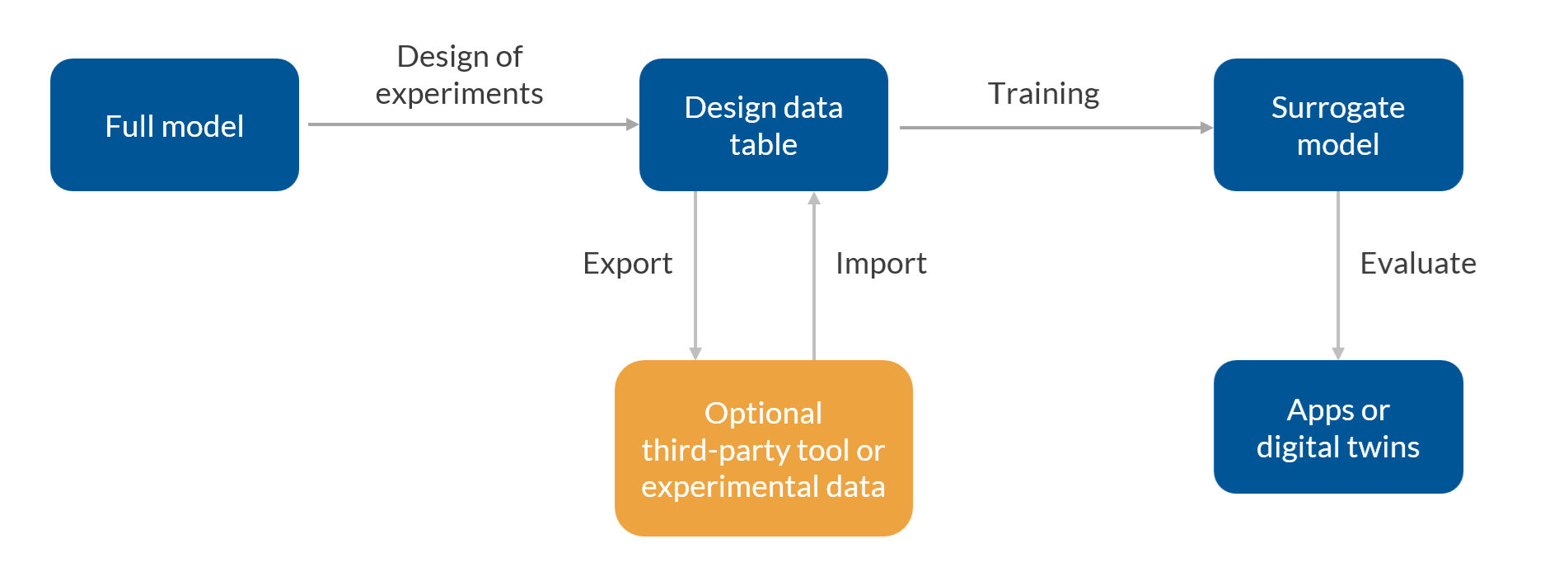 The workflow for using surrogate models.
Using Surrogate Models in Simulation Apps
One practical use of a surrogate model is to speed up a simulation app created with the Application Builder. In the example of the microstrip patch antenna app shown below, a function call to a surrogate model replaces the need to solve the full finite element model, resulting in near-instantaneous response times when varying the antenna’s dimensions or material properties. In the image below, we can see how the app displays the antenna gain pattern from the trained surrogate model, shown alongside the result from the original model for comparison.
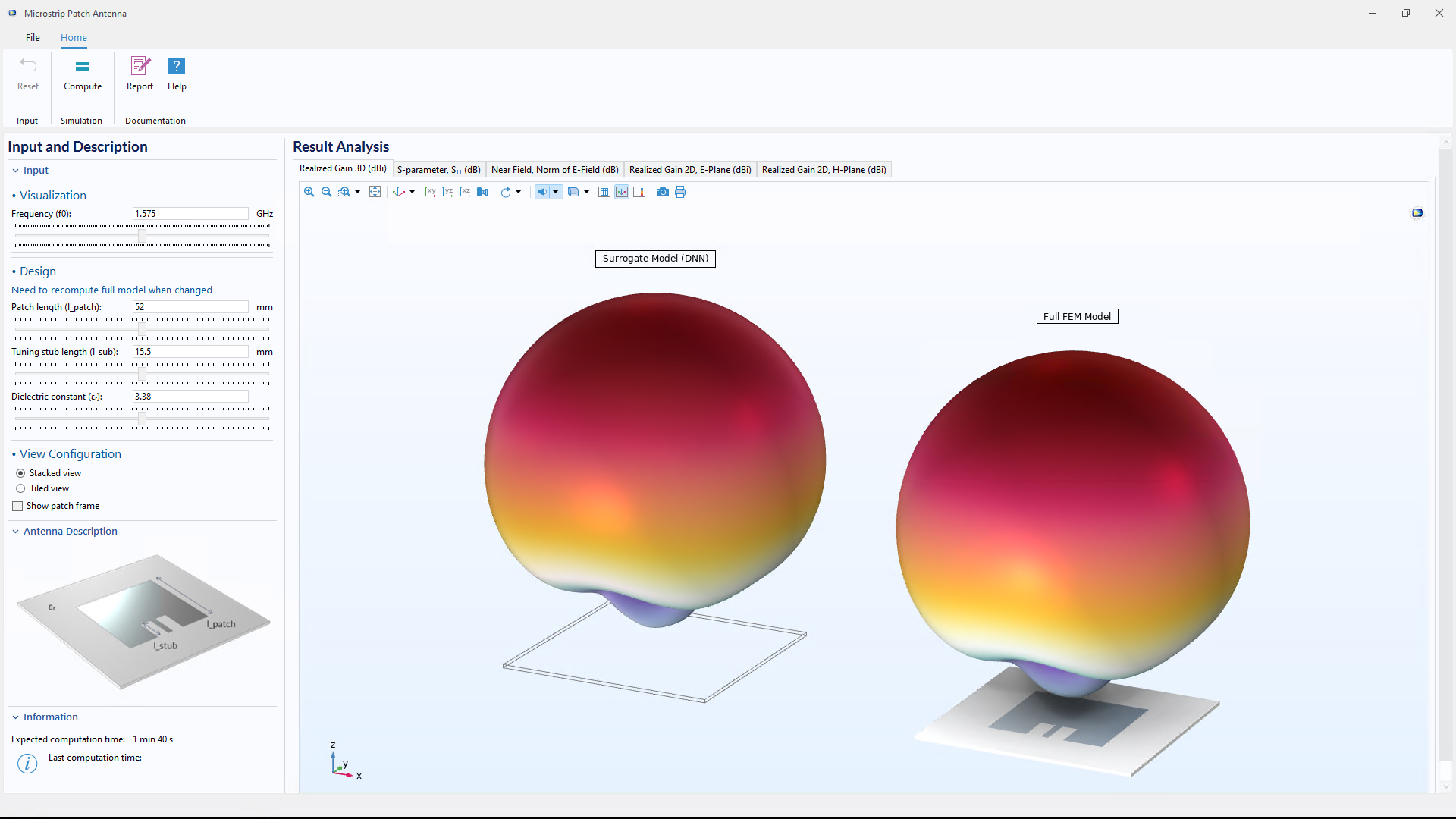 A simulation app comparing results from a surrogate model with those from a full simulation model.
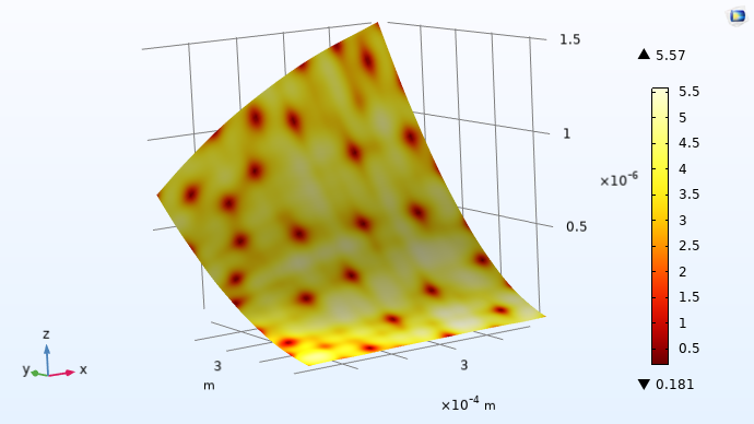
The image below shows another example of a simulation app that has been accelerated using surrogate models. In this case, a set of surrogate models is used to reconstruct the electric potential, temperature, and stress in a MEMS actuator. The user can interactively adjust four geometric dimensions of the CAD model, along with the applied voltage, using sliders. Thanks to the surrogate models, the app responds quickly, enabling a much more interactive experience than would be possible with a full simulation model.
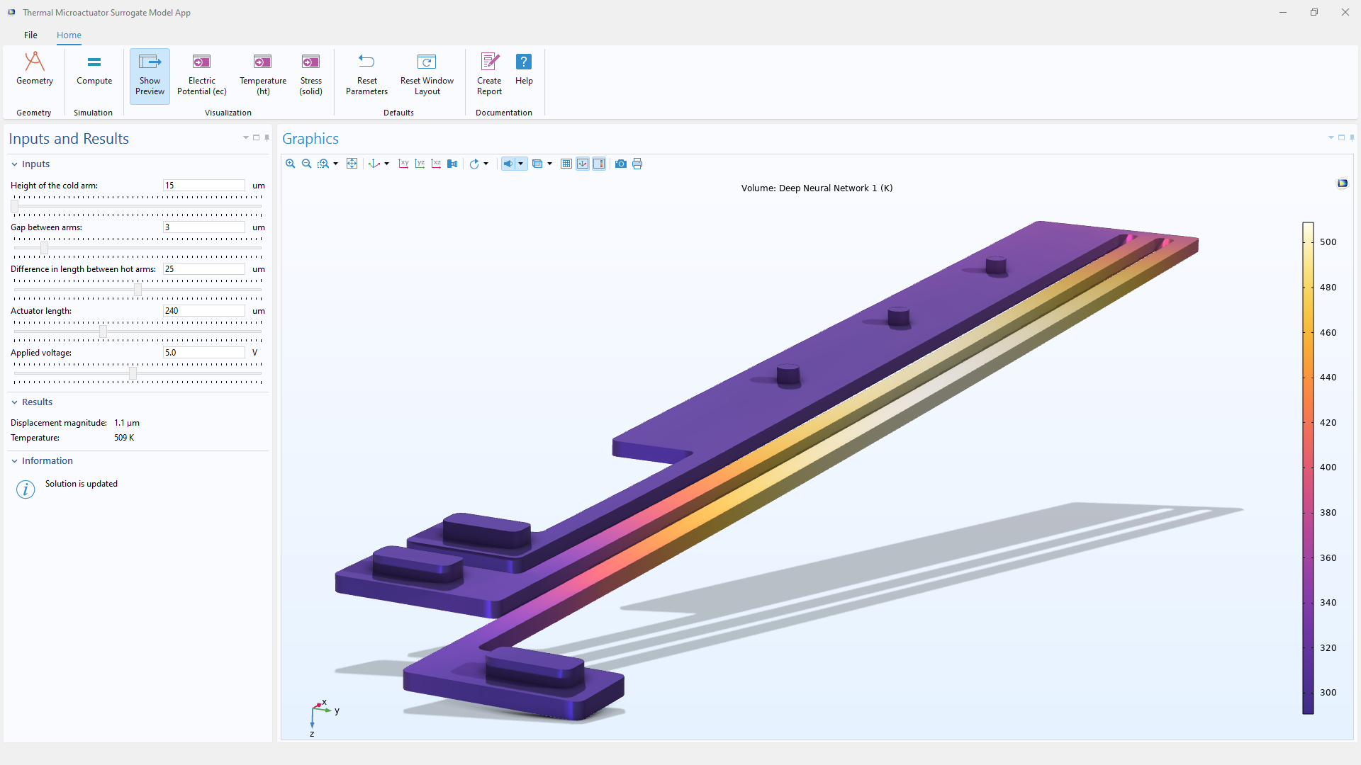
A simulation app of a MEMS actuator that uses multiple surrogate models to quickly visualize and evaluate physical field quantities such as the temperature, stress, and electric field.
In the MEMS app shown above, the visualizations and result evaluations are generated from a set of surrogate model functions that are called upon behind the scenes. A function corresponding to the temperature field is shown in the image below.
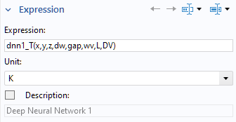 A function call to a deep neural network (DNN) surrogate model function, used behind the scenes in the MEMS app.
The syntax dnn1_T(x, y, z, dw, gap, wv, L, DV) calls a DNN function named dnn1_T, with the eight input arguments listed in parentheses:
- Three spatial coordinates: x, y, and z
- Four CAD dimensions: dw, gap, wv, and L
- The applied voltage: DV
This type of function call replaces calls to the field quantities defined by the full simulation model, which in this case is a finite element model.
Each surrogate model can define multiple functions, each with any number of input arguments. These functions typically represent physical quantities such as an electric field, temperature, or stress. Since surrogate model functions can be differentiated, they are well suited for use in gradient-based optimization workflows, such as inverse modeling, where sensitivities with respect to input parameters are required.
Types of Surrogate Models
There are three types of surrogate models available in COMSOL®: DNN, Gaussian process (GP), and polynomial chaos expansion (PCE). The DNN surrogate model is included in the platform product and does not require any add-on products. The GP and PCE surrogate models are part of the Uncertainty Quantification Module, where they are automatically created and trained using dedicated solvers or studies for uncertainty quantification. However, any of the three surrogate model types can be trained on any kind of simulation or experimental data.
 A response surface for a GP surrogate model showing the uncertainty estimate (standard deviation).
Once trained, surrogate models are available as functions under the Global Definitions node, ready to be used throughout the model. Each type of surrogate model comes with its own advantages. The choice of surrogate model depends on the problem at hand: DNNs are powerful for complex, high-dimensional problems with large training sets, while GP and PCE models are better suited when you need access to the confidence or uncertainty in a prediction.
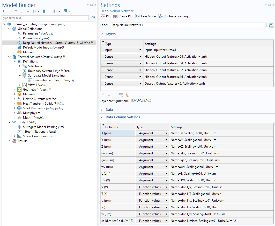 A DNN surrogate model definition that includes six functions in eight input arguments. The user interface makes it possible to customize the number of layers as well as the number of nodes per layer.
Note that for small datasets, GP models may be easier to create, and they perform better than DNN models.
Now let’s take a closer look at how the data used to train these models is generated.
Generating the Training Data
The Surrogate Model Training study is used to generate the data needed to train surrogate models. It performs a parametric sweep using methods based on DOE, and it can be configured to sweep over virtually any combination of input and output parameters. The result is a table of simulation data that serves as the basis for training. Surrogate models are not limited by physics; they can be used in applications across electromagnetics, structural mechanics, acoustics, fluid flow, heat transfer, chemical engineering, or any combination of multiphysics.
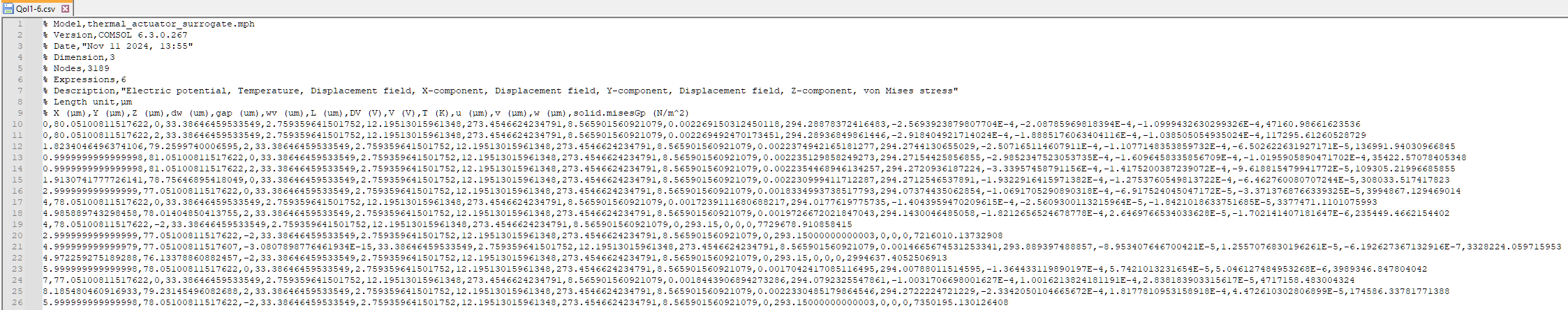 The first few rows of a data file generated by the Surrogate Model Training study.
Training Surrogate Models
Training is the step where the collected data is fitted to a surrogate model. Once trained, the surrogate model can be used in place of the original simulation, achieving significant speedup while maintaining sufficient accuracy in many cases. Surrogate models can either be trained automatically after the data generation step or added and trained manually in a separate step.
The fidelity of a surrogate model is controlled by the amount and quality of training data. A higher-fidelity model generally requires more data, which can be obtained from simulations, physical experiments, or a combination of both.
When working with surrogate models, the data-generation step is typically more time-consuming than the training step. However, both steps can be accelerated. Data generation can be sped up by running simulations on a cluster, allowing multiple design points to be computed in parallel. Training DNN surrogate models can also be accelerated using GPUs, which can significantly reduce training time for large datasets.
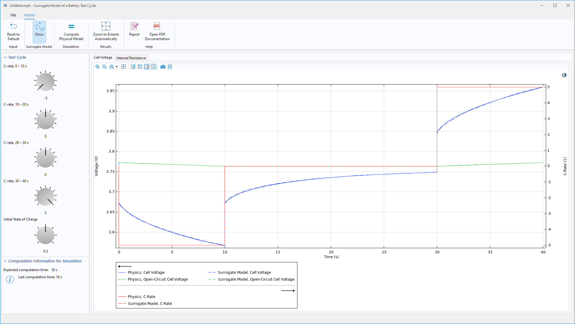 An app for analyzing the test cycle of a battery, highlighting how a DNN surrogate model can be used to reconstruct time-varying physical quantities.
Dive Deeper into Surrogate Models
In this blog post, we have provided a brief introduction of the functionality in COMSOL® for creating and building surrogate models. To get a more comprehensive overview of this functionality, check out our Learning Center course on surrogate modeling, which is an 8-part self-guided course that covers an introduction to creating surrogate models, fitting data with a DNN, evaluating model uncertainties, geometry sampling, and more.
Tip: To learn about the theoretical background of surrogate modeling, check out this Learning Center course: “Surrogate Modeling Theory”.


Comments (1)
Trevor Munroe
April 3, 2026Good brief blog. A contrast should be made between the differences in topology optimization results using the full model and the surrogate models.