
One of the common modeling situations that we encounter is the simulation of rotating objects exposed to loads. There are many ways in which such rotation can be modeled. In this blog post, we will look at addressing this by using the General Extrusion operators and discuss why this approach is useful.
A Practical Example: Cooking Meat by Rotation
There are many situations in which a rotating object is exposed to loads. For example, think of a rotisserie chicken or a kebab. Meat on a rotating spit is exposed to a heat load, usually a radiative heat source such as coals. Rotation is a simple way to distribute the applied heat. It keeps any regions from getting too hot or too cold and is an easy way to promote uniform cooking.
Now that I’ve got you licking your chops, let’s look at a slightly simpler case.
A Spinning Silicon Wafer Experiences Laser Heating
Today, we will look at the laser heating of a spinning silicon wafer. Although it isn’t quite as delicious to think about as rotating food, I’m sure you will find it equally informative.
As you may know, we already have an example of this in our Model Library and online Model Gallery. The existing example considers a wafer mounted on a rotating stage and heated by a laser traversing back and forth over the surface. The problem is solved in a stationary coordinate system. (Just think of yourself standing outside the process chamber and watching the wafer spinning on the stage.) We will call this the global coordinate system.
The laser is modeled as a heat source that moves back and forth along the global x-axis, while the wafer rotates about the global z-axis. The rotation of the wafer is modeled via the Translational Motion feature within the Heat Transfer in Solids physics interface, which adds a convective term to the governing transient heat transfer equation:
The right-hand side of the above equation accounts for the rotation of the wafer as \mathbf{u}, the velocity vector. This velocity vector can be interpreted as material entering and leaving each element in the finite element mesh — that is, we are solving a problem on an Eulerian frame. Since the geometry is a uniform disk and the applied velocity vector describes a rotation about the axis of the disk, this is a valid approach.
The drawback, however, is when you want to add more physics to the model. The Translational Motion feature is only available within the Heat Transfer physics and for many other physics interfaces that we do not want to solve on an Eulerian frame.
Instead of solving this problem on an Eulerian frame in the global coordinate system, we can solve this problem on a Lagrangian frame, with a rotating coordinate system that moves with the material rotation of the wafer. (Think of yourself as a tiny person standing on the surface of the wafer. The surroundings will appear to be rotating, whereas the wafer will appear stationary.)
The right-hand side of the above governing heat transfer equation becomes zero, but we now need to consider a heat load that not only moves back and forth along the global x-axis but also rotates around the z-axis of our rotating coordinate system. Although this may sound complicated, it is quite straightforward to implement.
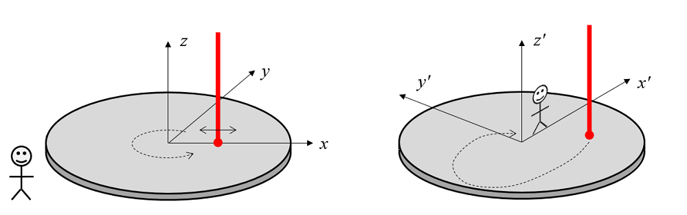
An observer in the global coordinate system sees a spinning wafer with a laser heat source traversing back and forth along the x-axis (left). An observer in a coordinate system rotating with the wafer sees the wafer as stationary, but the heat source moves in a complicated path in the x–y plane (right.)
Implementing Rotation via General Extrusion Operators
The General Extrusion operators provide a mechanism for transforming fields from one coordinate system to another. Some applications that we have already written about include submodeling, coupling different physics interfaces, and evaluating results at a moving point.
Here, we will use the General Extrusion operators to apply a rotational transformation to the applied loads. Our loads are applied in the rotating coordinate system via a coordinate transform from the global coordinate system given by the rotation matrix:
We can start with the existing Laser Heating of a Silicon Wafer example and simply remove the existing Translational Motion feature. We then have to add a General Extrusion operator, which implements the above transformation, as shown in the screenshot below. We will also want to implement a second operator that applies the reverse transform, which is done by switching the sign of the rotation.
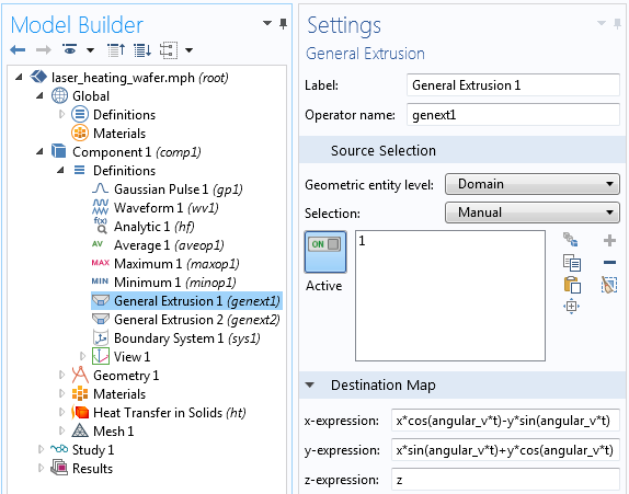
The general extrusion operation applies a rotational transform.
The applied heat load is described via a user-defined function, hf(x,y,t), that describes how the laser heat load moves back and forth along the x-axis in the global coordinate system. This moving load is then transformed into the rotating coordinate system via the General Extrusion operator, as shown in the screenshot below.
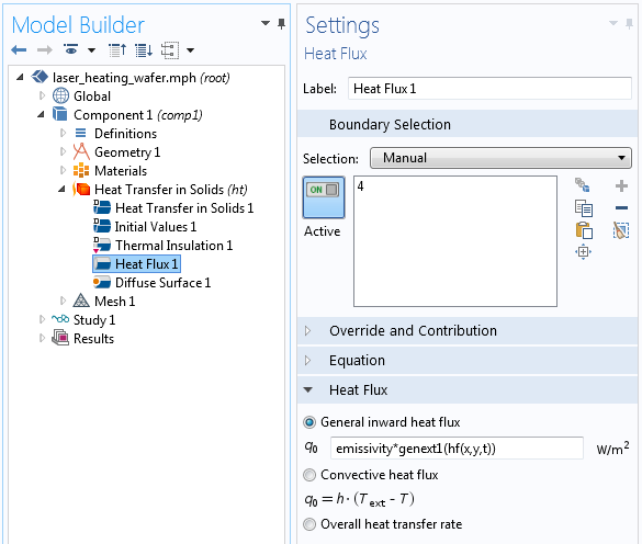
The applied heat load in the rotating coordinate system, defined via the global coordinate system and the rotational transform.
That’s it — you can solve the model just as before.
The results will now be with respect to the rotating coordinate system. It can be more practical for us to plot the temperature solution with respect to the global coordinate system by using the General Extrusion operator that applies the reverse transformation. This will give us a visualization of the temperature field as if we were standing outside of the process chamber and were watching the spinning wafer with a thermal camera.
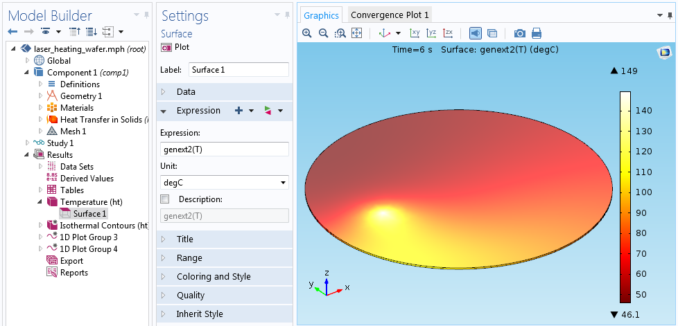
The second general extrusion operator is used to rotate the results back to the global coordinate system.
Concluding Remarks
The results of the simulation of the temperature field over time will be identical regardless of whether you use the Translational Motion feature or the General Extrusion operator. Although the General Extrusion operator requires more effort to implement — and does take a bit longer to solve — it is needed if you are interested in more than just the thermal solution.
For example, if you also need to compute a temperature-driven chemical diffusion and reaction process or the evolution of thermal stresses during the wafer heating, these problems should be solved on a coordinate system that rotates with the wafer.
There are of course many other applications where you could use the General Extrusion operator, but I hope I’ve satisfied your appetite for today!


Comments (5)
Vishwas Nesarikar
April 3, 2015You have lots of good blog examples of on your web site. However, if I want to separate the ones which are most useful for me after going through search, is there any way (similar to You Tube) create favorites list, so you can go directly to those you have book marked from previous searches ?
This will help reduce search time. Also, can the new posts be separated up front , if you happen to log in after brief break.
Thanks
Fanny Griesmer
April 6, 2015 COMSOL EmployeeHello Vishwas,
I am happy to hear you enjoy reading our blog.
We do not currently have the functionality you mention, but thank you for suggesting it to us.
ABDELKRIM MERZOUGUI
October 5, 2015thanks
Lyubo
July 19, 2020How can it be ablated?
Francisco Moraga
September 9, 2020I tried to use the general extrusion operator described above, genext1, to simulate a rotation with the only difference that instead of applying to a domain it was applied to a boundary. The idea was to take the boundary temperature of a previous steady simulation, comp1.T, and use it to put a rotating temperature boundary condition. Yet the mapping failed to reproduce the temperature on the boundary.
Is there a reason why the mapping can not be applied to a boundary?
If so, is it possible to adapt the idea to a boundary?
Or is the problem that if the mapping comp1.genext1(comp1.T) there is no clear definition of the time variable t in geneext1?