
Surface acoustic waves are capable of generating a streaming flow inside a droplet, enabling contactless mixing — a useful application in the area of microfluidics. Due to the multiphysics nature of the droplet streaming, a numerical study often makes several assumptions to capture only a part of the phenomenon. In this blog post, we will get the whole picture by modeling the streaming from the applied electric potential all the way to the generation of streaming flow using the COMSOL Multiphysics® software.
Inducing Streaming with Surface Acoustic Waves
When alternating voltage is applied on the surface of a piezoelectric material, it generates a strain determined by the electrical field, and waves start to propagate on the surface. These waves are called surface acoustic waves (SAWs), and they are distinguishable by how the material deforms relative to the propagation and normal directions. Two types of SAWs include Rayleigh waves and Love waves. This blog post will focus on Rayleigh waves, which make the surface deform in the normal direction. For the generation of the SAWs on the substrate, normally a set of comb-like terminals, or interdigital transducers (IDTs), is used to impose alternating electric potential. IDTs can both generate and receive the SAWs. When used as a filter in electric components, one more set of terminals is placed on the path of generated SAWs. The two terminals of the IDT on the receiver side will have different electric potentials according to the strain the substrate is experiencing, and information about the oscillation can be determined.
Instead of placing the second IDT on the surface as a receiver, we will put a droplet on the propagation path. The droplet will start interacting with the SAWs and absorb their energy. The SAWs attenuate as they travel under the droplet and are called “leaky SAWs” for this behavior. Energy is radiated to the droplet in the form of bulk waves incident at an angle called the Rayleigh angle. In the droplet, the incident waves reflect on the free surface of the droplet while also losing energy due to viscous dissipation, eventually resulting in a steady circulating flow component called acoustic streaming. We can induce steady flow just by oscillations. This plays an important role in the microfluidics area — we can enhance mixing inside the droplet without needing to physically put something in the fluid to stir it; the method is noninvasive. The resulting streaming may have different circulation patterns inside the droplet depending on the energy of the waves, the dimensions of the system, the material properties of the droplet, and so on.
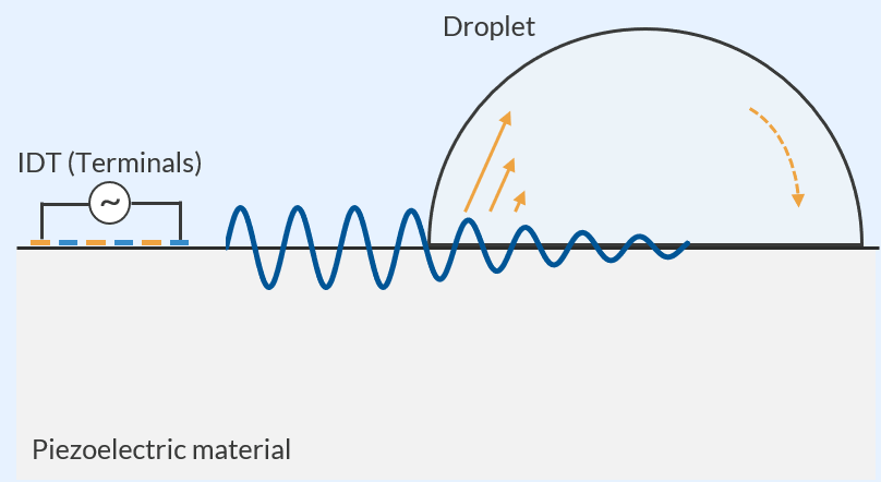 Schematic of SAW-induced streaming. The SAWs (wavy blue line) depart from the IDT. Once they reach the droplet, the energy is transferred into the droplet (solid yellow arrow), and finally, the streaming occurs (dashed yellow arrow).
As we have seen so far, the droplet streaming has multiple physics areas involved. Due to their complexity, these contributing factors are frequently modeled separately by dividing the process into several steps. Note that the analysis of the acoustic field in a droplet takes up considerable RAM (under the current conditions), while the analysis of the other fields usually does not. We will use COMSOL Multiphysics® to handle the complexity and create a model covering the whole process of transferring energy in the system. In this model, the drop has a wetting diameter of about 2 mm and a contact angle of 78° with the solid surface. The SAW device is excited with a frequency of 20.37 MHz. The droplet is assumed to be a glycerol–water mixture, and the properties of the piezo crystal are taken from the lithium niobate material in the Piezoelectric material library. As a reference, the values and setup are similar to the ones used in the paper: “On the Influence of Viscosity and Caustics on Acoustic Streaming in Sessile Droplets: An Experimental and a Numerical Study with a Cost-Effective Method” (Ref. 1).
Streaming Model Setup in the 2D Configuration
First, we will check what the model looks like in 2D. We know that the streaming has a 3D structure because of the hemispherical shape of a droplet, but it is always a good starting point to create a 2D model to see if the necessary settings and physics are complete and that the phenomenon we hope to model occurs under the 2D assumption. We will use the same cut plane as the schematic shown above for the 2D simulation. We will use the Electrostatics, Solid Mechanics, Pressure Acoustics, and Creeping Flow interfaces to excite the SAWs, and to capture the streaming, the Acoustic Streaming Domain Coupling multiphysics is used. Given that the time scales are quite different between the oscillation and the streaming, the simulation is done in two steps: a Frequency Domain study and a Stationary study.
In piezoelectric analysis, we need to pay attention to the crystal cut of the piezoelectric material. In this model, 128° YX-cut lithium niobate (LiNbO3) is used for the substrate; thus, the rotation should be reflected on the material properties. Functionality in COMSOL Multiphysics® enables us to consider the angle of the crystal cut by defining a coordinate system using, for example, the Rotated System feature and specifying the coordinate system in the Piezoelectric Material node of the Solid Mechanics interface. We also have an entry in the Application Gallery that explains the coordinate settings: Euler Angles Rotation in SAW Modeling. Note how the angles are set differently in the Application Gallery model for a 2D component (XY sagittal plane) vs. a 3D component (XZ sagittal plane). Further below, we will create a 3D model with the XZ plane as the sagittal plane.
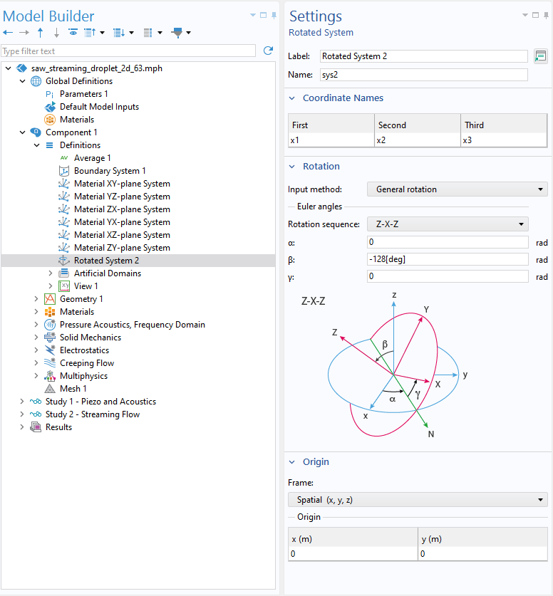 Settings of the Rotated System feature in the 2D model. In the 3D model, the value for β is set to -38 [deg].
We also need to make sure that an appropriate loss mechanism is taken into account in the Pressure Acoustics node. In the current setup, it is mostly the Eckart streaming that drives the flow inside the droplet. Therefore, the bulk attenuation of the sound wave should be modeled to capture it. The Fluid model in the Pressure Acoustics node specifies what type of attenuation the acoustic waves will experience. Here, we simply choose Viscous. If we left Linear elastic selected (the default), we would see no streaming in the results.
One last point to check is the Values of variables not solved for settings in the Stationary step. In the streaming analysis, the Acoustic Streaming Domain Coupling feature couples the Frequency Domain and Stationary studies. When the coupling is activated in a Stationary study, it refers to the variables solved in a Frequency Domain study to calculate the terms contributing to the streaming. Since we use multiple study nodes, the coupling does not know which solution has the frequency domain data of interest, so we need to specify it in the settings of the study step.
Now, let’s run the Frequency Domain and Stationary studies in order. The result should show distributions like the images below. The IDT is placed to the left of the droplet, outside of the images. There are SAWs generated on the piezoelectric material, moving to the right. The wave propagation direction can be checked more clearly using the Animation feature with the Dynamic data extension. The surface waves turn almost invisible after they have traveled over half of the contacting area. In exchange, the bulk waves in the droplet propagate in the upper-right direction, resulting in a complex pressure pattern. As might be expected, the circulating flow field is also confirmed from the stationary result. It has a large vortex across the whole domain area, but note that this might be 2D-specific. In a 2D configuration, we cannot simulate a vortex whose axis is not normal to the screen. However, it is a good start that we have set up a SAW model that induces streaming similar to what we have expected. Let’s move on to the 3D model.
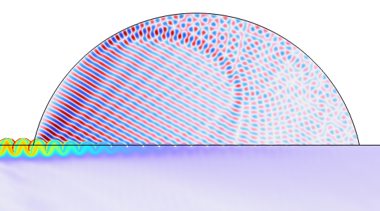
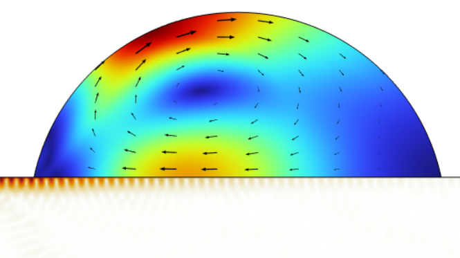
Results computed in the 2D model. Stress in the substrate and acoustic pressure in the droplet (left); displacement of the substrate and velocity distribution of the streaming in the droplet (right).
Tackling the RAM Issue in the 3D Configuration
Despite the difference in the dimension, from 2D to 3D, the principles of the simulation do not change. We use the same interfaces with the same multiphysics couplings. What does differ from the 2D model is the requirement for the computational resources. The 3D model’s geometry dimension is much larger than the wavelength, and it is highly likely to face memory issues. Not only would we experience longer computation, but we would also need to reduce the memory consumption so that the model can fit into the RAM of the computer.
First, we can simplify the geometry to an extent that will not significantly affect the result. In the 3D model, the IDT is modeled as several sets of simple rectangular 2D terminals that are placed in parallel. Moreover, the droplet and the substrate are cut in half by the middle plane to halve the degrees of freedom (DOFs). A periodic condition is used for the transverse direction of the piezo while a symmetry boundary condition is applied to the drop. This is a good approximation for the physics, especially when we are interested in the flow field in the droplet. We would need to widen the substrate domain if the model exhibited a strong dependency on the transversal length.
Second, considering that the resolution levels required to capture the waves are different in the droplet than in the substrate, we will use different mesh and mesh sizes for them. This is achieved by using the Form Assembly method instead of the Form Union method in the geometry sequence. This feature will allow the model to have multiple geometry objects in a component, mesh each object separately, and connect them using the so-called Pair feature that couples nonconforming meshes. Remember to use the Union operation where applicable so that the software can recognize that some of the geometry instances belong to a single object. The domains that belong to the same object will have a conformed mesh, and no pair is used between them.
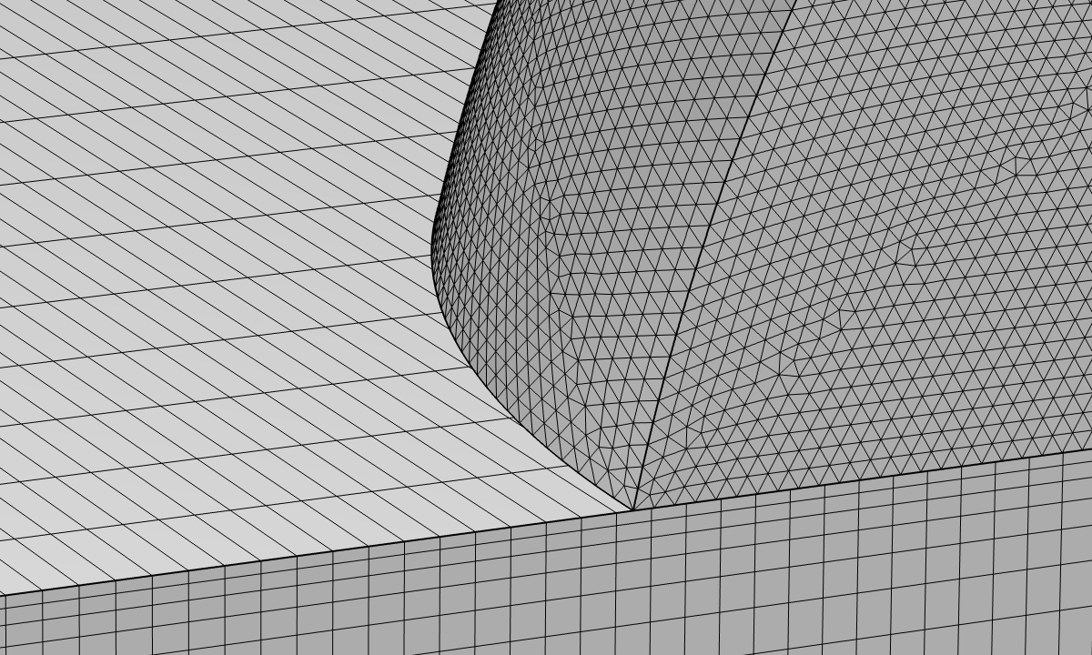 Magnified view of the nonconforming mesh near the leading edge of the droplet.
Lastly, we need to use an iterative solver to reduce the RAM usage in the Frequency Domain study. A general guideline on the settings of iterative solvers for acoustics problems is available in the Solving Large Acoustics Problems Using Iterative Solvers section of the Acoustic Module’s User Guide documentation. In this model, the number of DOFs for the Electrostatics and Solid Mechanics interfaces is much smaller than for the Pressure Acoustics interface, and direct solvers are expected to work well for solving for the electric potential and the solid displacement fields. Therefore, we activate hybrid preconditioners and use a Direct Preconditioner for the dependent variables of the Electrostatics and Solid Mechanics interfaces. With this feature, we can use a direct solver for small fields while applying efficient solvers to the other large fields. If the model did not have a piezoelectric domain, we could use a Segregated solver to reduce the RAM usage even further. However, as explained in Solving Large Acoustic–Structure Interaction Models section of the Acoustic Module’s User Guide documentation, acoustic–structure interaction models with piezoelectricity need to use the Fully Coupled solver, so the linear solver is the only part we can tweak. The acoustics part of the equations uses the shifted Laplace approach as an efficient form of the multigrid preconditioner.
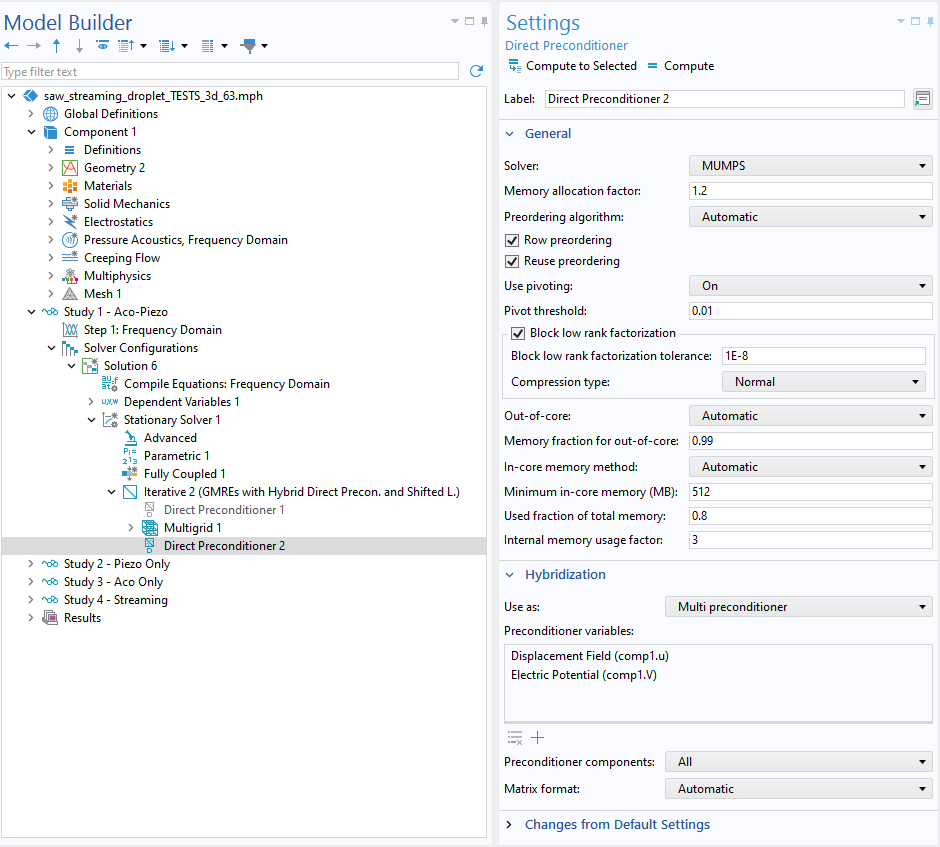 The Settings window for Direct Preconditioner in the 3D model. Note that hybridization is activated by choosing Multi preconditioner in the Hybridization section.
Now, the Frequency Domain study solves with 130 GB RAM in about 1 hour 10 minutes in our environment. However, even after running the study, there is something we need to keep in mind: rendering. In a large model, rendering a result can take a long time. To simplify working with large models, it is recommended that you enable the Only plot when requested checkbox in the Settings window for the Results node.
The results below clearly show the influence of the 3D geometry. Now the pressure pattern has a more defined peak in the middle slice than the 2D result. In addition, although it is a bit difficult to discern from a single picture, a small vortex is formed near the leading edge, and the rest of the droplet is occupied by a large vortex. These show good agreement with the reference, where a 3D simulation was conducted by decomposing the computation into 2D subproblems. In our model, we have been taking a rather straightforward approach; thus, we can simply set up multiphysics modeling with some modifications in the settings. The strategy to use the nonconforming mesh and the iterative solver would also work for other large problems, such as complicated MEMS devices.
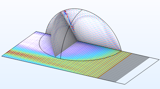
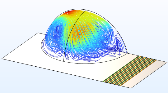
Results computed in the 3D model. Stress on the substrate surface and acoustic pressure in the droplet (left); streamlines of the streaming colored by the velocity magnitude (right).
Now It’s Your Turn
In this blog post, we have dealt with the complexity of modeling streaming in a droplet and the multiphysics involved using 2D and 3D models. We observed the interactions between physics interfaces, even with the 2D model, that solved quickly. Extending a 2D model to a 3D one can sometimes be challenging; it might require trial and error to see what configuration works for each model. We hope the current strategy will be useful to your multiphysics problem. The models are available from the following links:
As mentioned above, piezoelectric materials are frequently used to excite SAWs, but the definition of the properties requires special attention in terms of the coordinate system. Moreover, the design of the IDTs is closely related to the wave speed to excite; therefore, it is also important to see if SAWs are generated as desired. The following models work as useful references to test your SAW setup before building a complex model:
- Euler Angle Rotation in Surface Acoustic Wave Modeling
- Surface Acoustic Wave Velocity Calculations from a Unit Cell
This blog post does not mention particle movement in the streaming flow. To model acoustic manipulation of such things as particle movement, it might also be necessary to consider acoustic radiation force exerted on the particles. The Particle Tracing for Fluid Flow interface includes this functionality in the Acoustophoretic Radiation Force node, which can be used along with the Drag Force node. This combined use will consider the force due to the steady flow component at the same time. The following models would be useful as the starting point of such applications:
- Acoustic Streaming in a Microchannel Cross Section
- 3D Acoustic Trap and Thermoacoustic Streaming in a Glass Capillary
Reference
- A. Riaud et al., “On the Influence of Viscosity and Caustics on Acoustic Streaming in Sessile Droplets: An Experimental and a Numerical Study with a Cost-Effective Method,” Journal of Fluid Mechanics, vol. 821, pp. 384–420, 2017. DOI: https://doi.org/10.1017/jfm.2017.178


Comments (0)