
Electromagnetic Waves, Theory
Electromagnetic Waves in Media Without Free Charges
Maxwell's equations in a medium characterized by an electric permittivity,  ; magnetic permeability,
  ; and electric conductivity,
 , take the following forms in a medium without free charges:
| Equation Name | Differential Form | Comment |
|---|---|---|
| Maxwell–Ampère's law |  |
An electric field together with its rate of change generates a magnetic field. |
| Faraday's law |  |
The rate of change of a magnetic field generates an electric field. |
| Gauss's law |  |
The assumption is that there are no free electric charges. |
| Gauss's magnetic law |  |
There are no free magnetic charges. |
Maxwell–Ampère's law and Faraday's law can be combined into a second-order wave equation by taking the curl of one equation and substituting it into the other. In other words, the system formed by these two first-order equations represents electromagnetic waves.
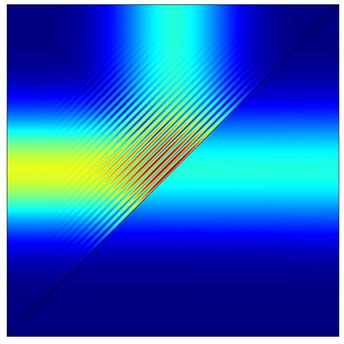
Beam splitters can split a beam of light, such as one with a 700-nm wavelength, into two. To create a beam splitter, one method is depositing a layer of metal between two prisms made of glass. Within the layer, the beam is attenuated slightly and then separates into two different paths. The image shows the magnitude of the electromagnetic wave, where red and blue are high and low values, respectively.
Beam splitters can split a beam of light, such as one with a 700-nm wavelength, into two. To create a beam splitter, one method is depositing a layer of metal between two prisms made of glass. Within the layer, the beam is attenuated slightly and then separates into two different paths. The image shows the magnitude of the electromagnetic wave, where red and blue are high and low values, respectively.
Field Formulations for Electromagnetic Waves
To derive a single second-order wave equation for the electric field, first assume that the material is time invariant. The permeability can then be taken outside of the time derivative in Faraday's law and inverted:

Now, take the curl of this equation:

Collecting terms on one side gives:

A similar derivation gives the following equation in terms of the magnetic field:

With this formulation, we have assumed space-independent material properties. By instead deriving a wave equation from the magnetic vector potential, this restriction can be relaxed, as shown below.
Electromagnetic Waves in Free Space
In free space, ,
, , and
, and  . The equation for the electric field can be put on the form:

An equivalent formulation is:

where the speed of light is:

Gauss's law in free space is  , which together with the vector identity:

gives the following, and perhaps more familiar, form of the wave equation:

and similarly gives the following form for the magnetic field:

Electromagnetic Wave Equations
The most important equations for electromagnetic waves are summarized in the following table:
| Equation Name | Differential Form | Integral Form | Boundary Condition |
|---|---|---|---|
| Gauss's magnetic law |  |
 |
 |
| Maxwell–Ampère's law (magnetostatics) |  |
 |
 |
| Faraday's law |  |
 |
 |
Here,  is the magnetic flux through the closed contour C, while
  is the surface current density.
The limiting process for deriving the boundary conditions corresponding to the surface integrals in Maxwell–Ampère's law and Faraday's law involves fluxes that run perpendicular to the limiting surface. The process's contribution is zero for a vanishing surface area, and because of this, the boundary conditions corresponding to Maxwell–Ampère's law and Faraday's law are identical to those of the static cases.
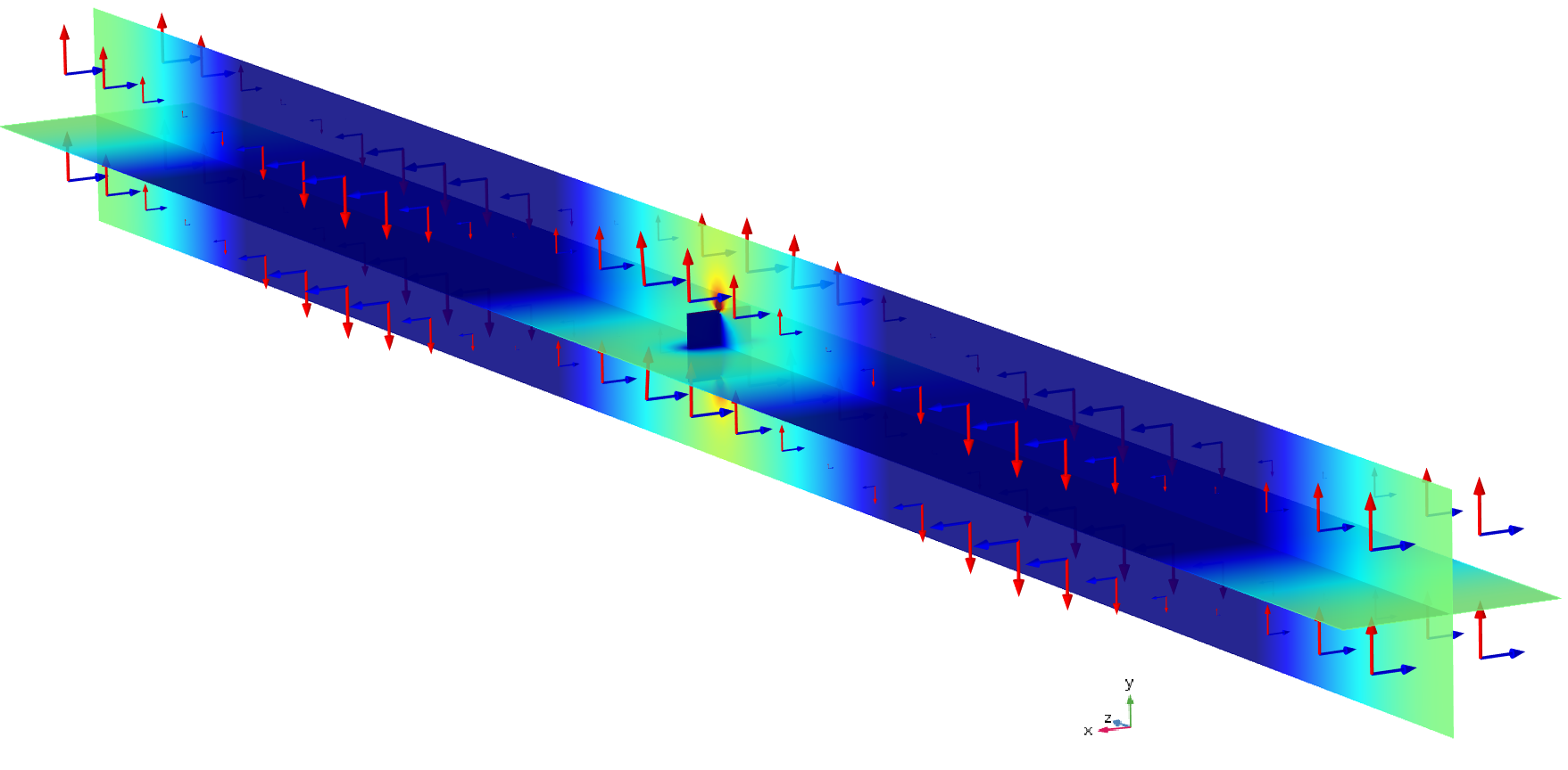
A section of air surrounding a rectangular, perfectly conducting metallic plate subjected to an incident plane electromagnetic wave at 10 GHz. The plate is 1.5 by 1.5 by 1 mm. The electric and magnetic vector fields are represented by red and blue arrows, respectively. The electric field is polarized in the y direction. The  -component of the field is visualized at a certain instance in time by color on two intersecting planes, where blue and red represent low and high field values, respectively. The field pattern near the plate is a result of the fact that the electric field tangential to the metallic plate is zero.
A section of air surrounding a rectangular, perfectly conducting metallic plate subjected to an incident plane electromagnetic wave at 10 GHz. The plate is 1.5 by 1.5 by 1 mm. The electric and magnetic vector fields are represented by red and blue arrows, respectively. The electric field is polarized in the y direction. The -component of the field is visualized at a certain instance in time by color on two intersecting planes, where blue and red represent low and high field values, respectively. The field pattern near the plate is a result of the fact that the electric field tangential to the metallic plate is zero.
Vector Potential Formulation for Electromagnetic Waves
It is possible to derive a second-order wave equation by means of the magnetic vector potential. To do so, start by assuming the temporal gauge,  , together with the definition of the vector potential,
 , and substitute them into Maxwell–Ampère's law:

Collecting terms on one side gives:

Note that this formulation is for a time-independent material. For a time-dependent material, the permittivity cannot be taken outside of the time derivative.
Time-Harmonic Formulations
A time-harmonic field,  , can be expanded as:

as can  and
and  , where higher-order terms include the overtones proportional to
  ,
,  , etc.
For a sinusoidal field, the overtones vanish and only the zeroth (constant) and first-order Fourier terms remain.
When manipulating expressions and equations involving time-harmonic fields, the time-independent part,
, etc.
For a sinusoidal field, the overtones vanish and only the zeroth (constant) and first-order Fourier terms remain.
When manipulating expressions and equations involving time-harmonic fields, the time-independent part,  , is seen as a complex-valued phasor field. The transformation back from phasor field formulations to real-valued, time-dependent quantities is:

The time-harmonic electromagnetic wave formulations are as follows:


Note that the equation for is identical to that of due to the relationship  .
.
Complex-Valued Permittivity and Refractive Indices
In optics, the refractive index,  , is the preferred material property. The refractive index is defined as:

where  is the speed of light in a vacuum and
  is the phase velocity of light in the medium.
The refractive index can also be written as a function of the relative permittivity, , and permeability,
  , according to
  .
.
In many important optical materials , is close to 1 and the refractive index is approximated as:

To model damping in the time-harmonic electromagnetic wave formulation, we can allow for a complex-valued permittivity (see also: Electroquasistatics, Theory and thereby a complex-valued refractive index:

Plane Wave Form of Maxwell's Equations
A plane wave expressed in a time-harmonic electric field can be written as a complex-valued phasor field:

where  is a constant vector;
  is the wave vector;
  is the spatial coordinate; and
  is the time-independent, complex-valued phasor field.
The condition that the wave is planar corresponds to  for the phasor field , assuming an isotropic material.
Faraday's Law
For a linear medium, the time-harmonic version of Faraday's law takes the form  .
.
For a plane wave, we have the following vector identity:

so that Faraday's law for a plane wave becomes  , or equivalently,
  .
.
Maxwell–Ampère's Law
The time-harmonic version of Maxwell–Ampère's law for a linear medium is:

For a plane wave in a medium with an isotropic homogeneous permeability, this equation becomes:

or:

The Plane Wave Equation
Now, write:

and combine into:

Some manipulation gives:

or:

Collecting terms on the left-hand side give:

For a material with  , the equation becomes:

This is the plane wave equation, which is restricted to media with a homogeneous isotropic permeability, as explained below.
Alternatively, it is possible to introduce a complex-valued permittivity:

In this case, the plane wave equation takes the following form:

Constitutive Relationships and Transverse Fields
If the medium has an anisotropic permeability, , then due to  , we may have that and
  are not aligned. Thus,
  , , and are not necessarily mutually perpendicular.
On the other hand, and are always aligned for a medium with an isotropic homogeneous permeability. Due to Gauss's magnetic law, , it holds that:

so that is guaranteed to be perpendicular to both and .
Furthermore, since  and , we have that is perpendicular to both and .
However, if we allow the permittivity to be anisotropic, then and  may not be aligned, as
  . This means that may not be perpendicular, or transverse, to .
Misaligned and or misaligned and corresponds to the wave vector not being aligned with the Poynting vector,  . Equivalently, the momentum flux
  is not aligned with the Poynting vector.
Last modified: February 13, 2019