
Many antennas deployed in basic communications systems are linearly polarized, meaning that for the orientation of the electric field, polarization is confined to a single plane. Antennas that present the option of circular polarization give you more to work with, because the polarization of the wave varies while it propagates. Helical antennas, for instance, are able to generate circularly polarized waves in the axial operating mode. RF simulation can be used to optimize helical antenna designs.
An Upward Spiral: The Growing Number of Helical Antenna Applications
Helical antennas are named for their spiral geometry, consisting of one or more conducting wires wound in a helix. Due to their shape, helical antennas are able to emit circularly polarized fields. Their design is simple but effective and can be applied in a variety of ways, including in highly compact antennas for use in smart implants and other RFID devices.
Larger helical antennas are used in radio, GPS, and ballistic missile system applications, as well as extraterrestrial communications with satellites and space probes orbiting Earth and the moon.
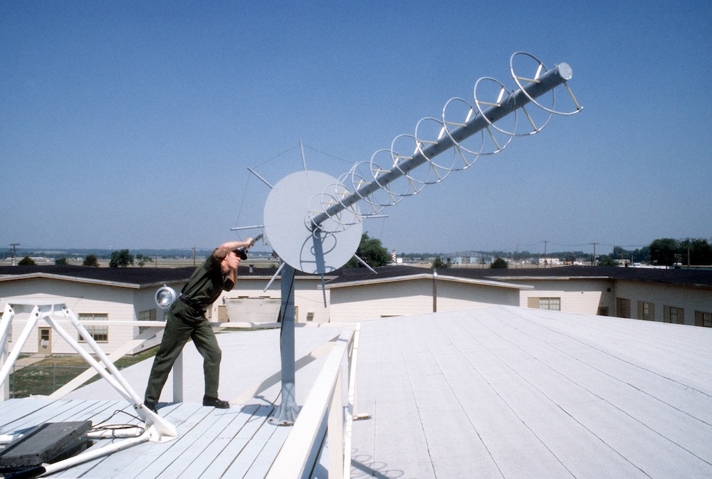
A helical antenna used for SatCom. Image in the public domain in the United States, via Wikimedia Commons.
One current project is boldly taking a helical antenna where no helical antenna has gone before: Mars. NASA’s “Interior Exploration using Seismic Investigations, Geodesy and Heat Transport (InSight)” mission aims to study Mars’ interior structure, including its crust, mantle, and core. The Mars lander will gather surface data, such as temperature and heat flow, to provide scientists with more insight into how rocky planets form. Among other instruments that measure and transmit information, the lander is equipped with a helical UHF antenna, which will be used for communication with orbital relay spacecraft.
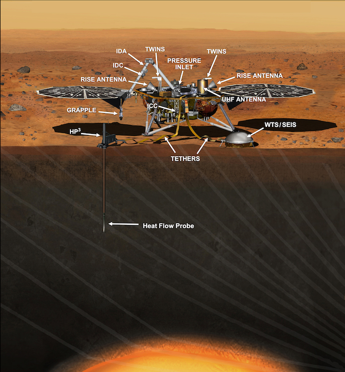
An artistic depiction of the InSight Mars lander. Image by NASA/JPL-Caltech. Image in the public domain in the United States, via Wikimedia Commons.
Optimizing helical antenna designs for these applications requires an understanding of their operating modes. This can be accomplished using RF simulation.
Helical Antennas: Two Operating Modes
Helical antennas can be set up with two arms (conducting wires) to account for their two major operating modes:
- Normal
- Axial
Similar to a monopole antenna, the normal-mode antenna is linearly polarized, but because it’s in a helical shape, it’s shorter and more compact. The antenna is considered a normal-mode helix when the circumference of the helix is significantly less than the wavelength and its pitch is significantly less than a quarter wavelength. In the normal, or perpendicular mode of radiation, the antenna’s far-field radiation pattern is similar to the torus-shaped pattern of the classic dipole antenna.
In the axial, or end-fire, mode of radiation, the antenna radiates circularly polarized waves. One of the benefits of circularly polarized waves is that they are less vulnerable to multipath fading and have less polarization dependency than linearly polarized waves. The antenna is considered an axial-mode helix when the helix circumference is near the wavelength of operation. The helical antenna is at a much higher frequency band than at the normal mode, working similarly to an end-fire array along the helical axis, generating a directive radiation pattern.
Impedance-Matching Ability, as in a Folded Dipole Antenna
An advantage of helical antenna designs with two arms is the ability to match impedance. With a single-helix antenna, the impedance is much lower when it is resonant at the normal mode. If you add a second antenna that is shorted to the ground, it acts as a folded antenna that has an input resistance four times bigger than a dipole antenna of the same size, which means that you can adjust the low impedance close to the reference impedance of the coaxial cable, 50 Ω.
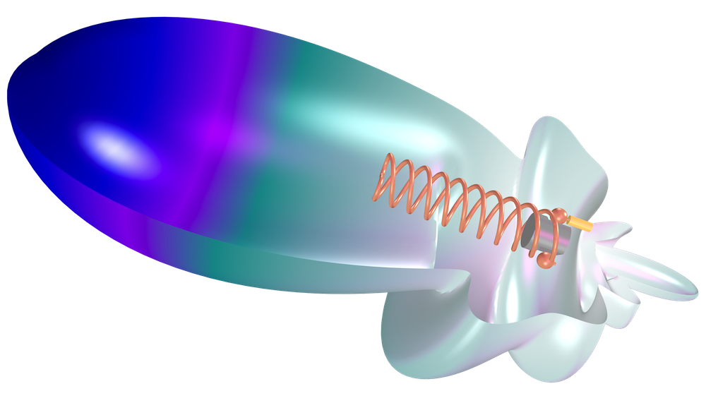
A model of a two-arm helical antenna and its axial mode radiation pattern. Only a half of the radiation pattern is visualized.
Simulating a Two-Arm Helical Antenna in the COMSOL Multiphysics® Software
This example of a two-arm helical antenna is modeled using the RF Module, which is an add-on to the COMSOL Multiphysics® software.
As shown below, the model geometry includes a two-arm helix radiator, a circular ground plate (shown in blue), a tuning stub, a coaxial cable, and a perfectly matched layer (PML) enclosing the air region. In addition, two helix structures are wound along the z-axis and meet at the top end.
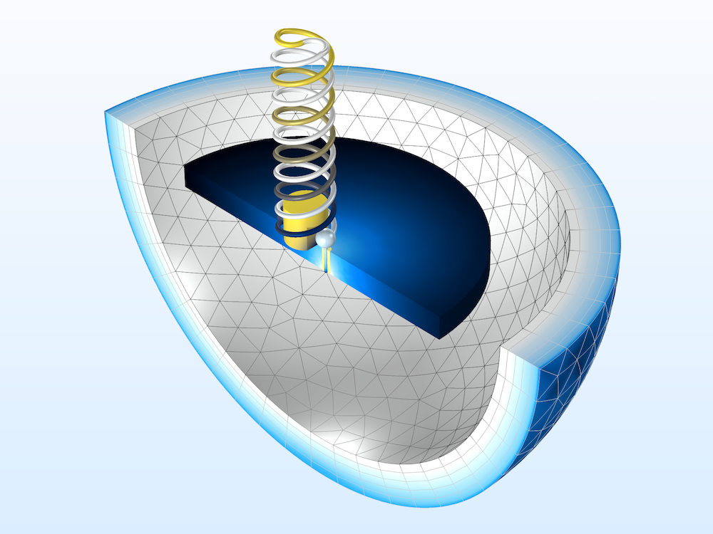
For this example, all metal parts are modeled as perfect electric conductors (PECs) and the space between the inner and outer conductor of the coaxial cable is filled with polytetrafluoroethylene (PTFE). To excite the antenna, a coaxial-type lumped port is used. In addition, all domains are meshed (except the PML) by a tetrahedral mesh with around five elements per wavelength, and the PML is swept along the absorbing direction automatically through the physics-controlled mesh.
In addition to the second antenna, which helps adjust for impedance, you can also add an impedance-matching stub for the axial mode located at the center of the ground plate. Note that the ground plate, the PML sphere shell, and the maximum mesh size are adjusted automatically as a function of wavelength for each operational mode.
Studying the Simulation Results
The S-parameters and far-field patterns are calculated at both of the operating modes: 0.385 GHz at the normal mode and 4.77 GHz at the axial mode. The results shown below plot the log-scaled electric field magnitudes for each mode. You can see a difference in field intensity around the antenna between the normal mode (left) and the axial mode (right).


Log-scaled electric field magnitude around the antenna at 0.385 GHz (normal mode, left) and 4.77 GHz (axial mode, right).
Next, let’s take a look at a polar plot of the 2D radiation patterns in the yz-plane. This plot shows both modes of operation. As expected, you can see a classic E-plane pattern of a dipole antenna at the normal mode (blue) and a directional radiation pattern at the axial mode (green).
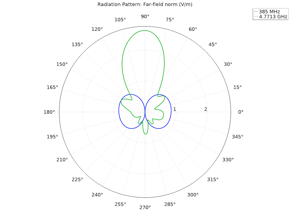
Polar plot of the far-field pattern in the yz-plane, with the normal mode shown in blue and the axial mode shown in green.
You also get a visualization of the radiation patterns in a 3D far-field radiation plot for each mode. The S-parameters for both modes are less than -10 dB. When you look at the 3D far-field patterns, these results once again verify the dipole antenna shape for the normal mode and the end-fire array shape for the axial mode.


The 3D far-field pattern at the normal mode (left) resembles that of a dipole antenna. The 3D far-field pattern at the axial mode (right) resembles that of an end-fire array antenna along the z-axis, backed by a ground plane.
Below, the axial ratio plot shows how much the antenna is circularly polarized. When it is characterized as the perfect circular polarization, the axial ratio is 1 or 0 dB. When it is below 3 dB (inside the red circle), it is typically regarded as a circular polarization. In the figure, the axial ratio is lower than 3 dB at the antenna boresight that is the major direction of propagation of the axial mode, parallel to the helical twist axis.
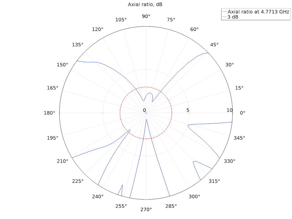
Axial ratio in dB scale (blue) plotted with 3 dB line (red).
By modeling a two-arm helical antenna, you can effectively analyze the normal and axial operating modes, which can help you improve antenna designs for terrestrial and extraterrestrial applications.
Next Steps
Want to try modeling a helical antenna? Get started by clicking the button below.
Further Reading
To learn more about antenna modeling, check out these blog posts:


Comments (0)