
One of the challenges when modeling inductive heating processes in 3D is that you often need to resolve the skin depth within the part being heated via a thin boundary layer mesh, but don’t want to include the remaining interior of the part within the electromagnetics model. Here, we will look at a meshing technique that efficiently addresses such cases.
Introduction to the 3D Inductive Heating Model
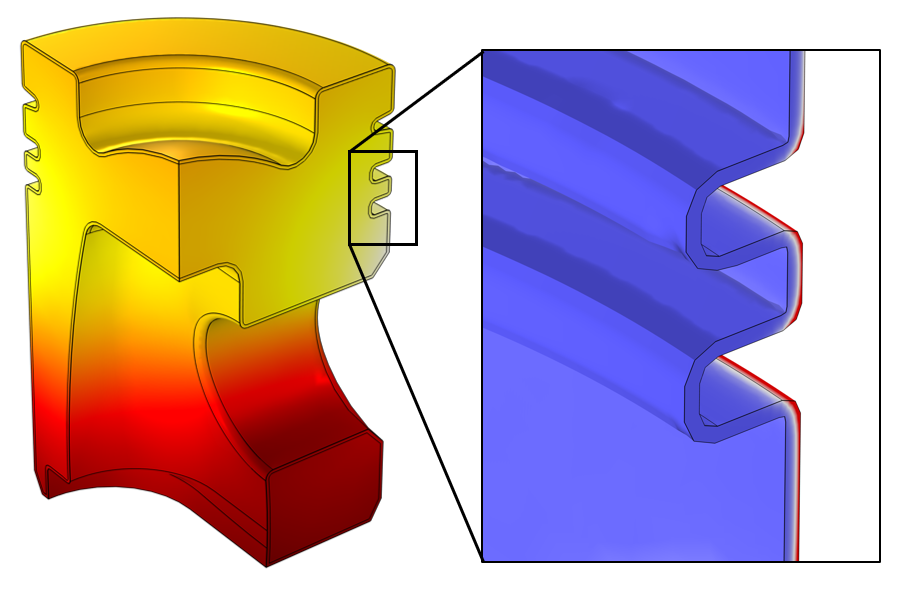
Consider the inductive heating setup shown in the image below, of a coil about an aluminum automotive piston head. For our purposes, we can assume symmetry and reduce the model to a quarter section, with Magnetic Insulation boundary conditions on the symmetry planes. We also approximate the boundary to free space via the Perfect Magnetic Conductor condition.
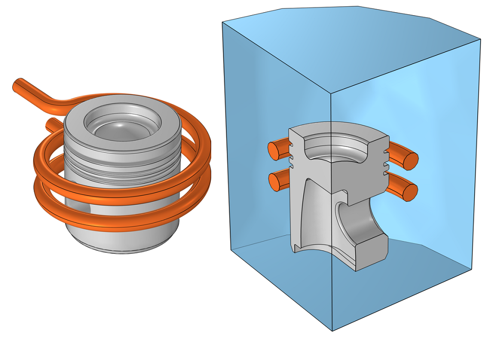
Inductive heating setup of an aluminum cylinder head and a corresponding computational model exploiting symmetry.
The inductive copper coil, operating at 40 kHz, can be modeled via two homogenized multiturn coils, which do not need to be very finely meshed. However, within the aluminum piston head, the skin depth is comparable to the smaller feature sizes, thus we know that we need to use boundary layer meshing to accurately compute the losses.
Since we know that the electromagnetic fields will not penetrate very far into the material, we would ideally like to omit all of the central volume of the part from the electromagnetic field calculation. On the other hand, we do know that the central volume of the cylinder will affect the thermal solution, so we cannot just remove that volume entirely. We need to partition our part into two subdomains, based on the boundary layer meshing requirements. As it turns out, a combination of meshing tools can be used to quickly and easily set up exactly such a model. Let’s learn more!
Efficiently Setting Up the Model and Mesh
Starting with the geometry pictured above, we define the mesh. We start by generating a tetrahedral mesh within the part and the surrounding air, and we define a boundary layer mesh, composed of four elements each equal to half the skin depth, on the exposed boundaries of the piston, as visualized in the images below.
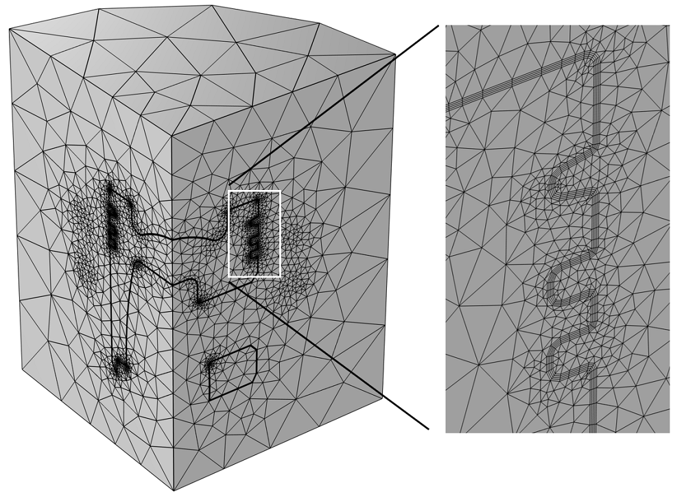
Mesh, with a highlight of the boundary layer mesh on the piston faces.
Once this mesh is built, we would like to partition the geometry up, based on the boundary between the skin depth mesh and the remaining volume within the part. This requires a few extra steps. First, we need to introduce another 3D Component into our model. Into the Mesh branch of this new 3D component, we will import the mesh that was created earlier.
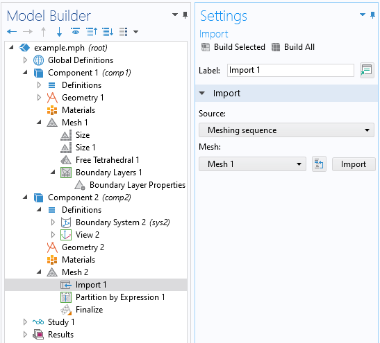
The import mesh operation that copies the mesh from one Component to the other.
After the mesh is brought into this new Component, we need to introduce a Partition feature into the mesh and partition via the expression: isprism, as illustrated in the screenshot below. The isprism variable is a logical variable that is true for only the prismatic elements used within the boundary layer mesh. This operation thus divides the meshed volume of the cylinder into two volumes:
- The thin shell that is meshed with prism elements
- The remainder
These different domains are available for when we start to add physics to the model. If we ever want to go back and modify the mesh, we will want to go back to Component 1, modify the mesh, and then reimport the mesh into Component 2. It’s important to note that you can’t add an additional geometry into Component 2 — You always have to go back to the original Component, modify the source mesh, and then reimport.
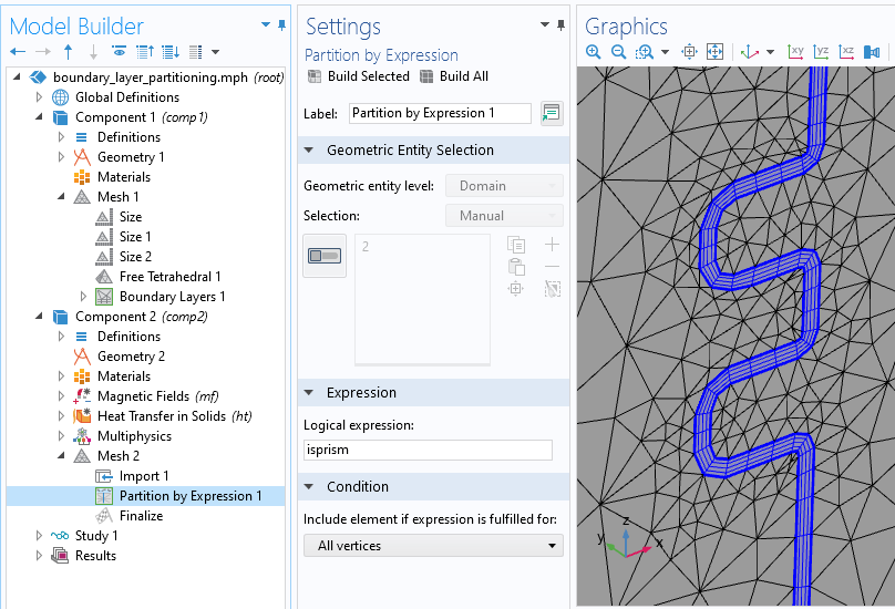
The Partition operation, operating on the mesh itself, along with a visualization of the newly created domain.
With this done, it’s possible to solve in the second Component for the electromagnetic fields in just the coil, air, and the boundary layer, while solving for the temperature field throughout the volume of the part. At the boundary between the boundary layer domain and the remaining volume of the part, it is reasonable to apply the Impedance boundary condition, as this will account for any small fraction of the losses that aren’t completely captured within the boundary layer mesh.
For this case, the electromagnetics model of just the coil, air, and skin depth region has ~20% less degrees of freedom than if we also solved for the fields deep within the part, which we already know are insignificant. These savings can be even more considerable for other parts.
The temperature field, computed throughout the volume, as well as the inductive heating, computed only within the boundary layer domain.
Further Resources and Closing Remarks
Find a comprehensive overview of modeling of induction heating and boundary layer meshing in this Learning Center course. The study type to use depends on the nonlinearities present, and if you want to study the temperature rise or the steady-state temperature field, as described in this previous blog post.
The technique shown here, of partitioning based upon the mesh, can be used in many other cases. It is even possible to reimport the resultant mesh as a geometry back into yet another component and remesh. Keep in mind, however, that the boundary layer meshing is an approximation of a uniform surface offset, and that the resultant geometry might not always be suitable for further geometric operations. As an alternative, if an exact offset is required and if robust subsequent geometry operations need to be performed, use the Thicken operation, which is available with the Design Module. However, in situations when an approximate thickness geometric layer is all that is needed, such as for 3D induction heating, the technique described here can be quite helpful.
Try It Yourself
Download the model file associated with this example by clicking the button below.


Comments (4)
Julian Anaya
May 12, 2021This is a very good trick indeed; however, I would say that this is only valid if the material we are heating is not ferromagnetic. If the permeability of the material depends on temperature this trick cannot be used and the full model must be used since the absorption of the energy is not ensured to happen very close to the boundary. E.g. if we have a piston made of mild steel and the temperature goes above the curie temperature then the region of high absorption of the energy moves to the interior of the piston as the permeability near the surface drops to 1.
Walter Frei
May 13, 2021 COMSOL EmployeeHello Julian,
I would agree, this approach is likely not very suitable for ferromagnetic materials. (We use here the case of an aluminum cylinder.) I should add that this technique (of creating a new component and partitioning the original mesh based upon element type) is almost certainly not solely applicable for inductive heating cases. Sometimes, within our blogs, we present techniques in the context of a specific situation, but often it is more the modeling technique, rather than the particular physics situation, that we’d like people to remember.
Ivar KJELBERG
May 12, 2021Hi Walter,
Nice Blog 🙂
I’m missing a comment on the HT part.
If the heating is “fast”, we would observe quite some steep Grad(T) and for that we need to ensure a fine mesh too such to resolve T in this critical region, particularly if we are in the time domain study.
Clearly the Boundary Mesh required here for the EM skin effect will help but one should check the Heat diffusivity of the heated material
alpha_th = k[W/(m*K)] / ( rho[kg/m^3] * Cp[J/(kg*K)] ) [m^2/s]
and compare to the local mesh size “h” as well as the time stepping Dt used by the solver, else the results would be wrong.
It will probably not be significant for a stationary solution, still worth to be reminded for any temporal solution.
Sincerely
Ivar
Walter Frei
May 12, 2021 COMSOL EmployeeHello Ivar, Yes, that is a good point. I think that (at least for a lot of cases of metals) if you’re refining the skin depth well with the mesh, you have a mesh that is “practically fine enough” for the thermal problem. Of course, yes, if you have a very fast transient, or some more exotic materials, then things may be different. That being said, your fundamental point is of course correct: A finite element analyst must always perform a mesh refinement study (https://www.comsol.com/support/knowledgebase/1261) to gain confidence in their results.