
Estimating Hyperelastic Material Parameters via a Lap Joint Shear Test

Guest blogger Björn Fallqvist from Lightness by Design returns to discuss different methods for hyperelastic material analysis, including lap joint shear tests and damage models.
This two-part blog post demonstrates a simple lap joint shear test that can be used to determine material parameters for polymers. A follow-up post will propose a physically motivated damage evolution law for the material.
Introduction
For many soft materials, especially rubber and biological tissues, the relationship between stress and strain is not linear, even at small loads. The microstructure of these polymer materials gives rise to its nonlinear behavior. For example, in materials such as biopolymer networks, the polymer chains are entangled and often cross-linked. The macroscopic material response then depends on several different mechanisms. Among these can be mentioned the sliding of filaments due to thermal exchange, entropic stiffness from filament straightening, and cross-link stiffness (as well as debonding).
Naturally, this complex behavior results in that the often-used idealization of the material as linear elastic is not valid, and a different approach to its modeling must then be taken. Typically, one does this by choosing a hyperelastic model, in which a strain-energy density function can characterize the state of the material and the associated stresses.
There are many forms of hyperelastic functions to choose from, and in all cases, an analysis involves determining at least one material parameter. Finding these requires the use of experimental data. A previous COMSOL blog post describes this in detail (Ref. 1). However, the data for different deformation states are often either not available or expensive to obtain.
The simple lap joint shear test can be used to determine these material parameters for polymers, and this blog post demonstrates a method to do so.
Modeling Hyperelastic Materials
Hyperelastic materials can be modeled by postulating the existence of a strain energy density function:
which is a function of the deformation state, here symbolized by the deformation gradient \mathbf{F}.
By differentiating \psi with respect to the right Cauchy–Green tensor \mathbf{C}, one obtains the second Piola–Kirchhoff stresses \mathbf{S}, which can thereafter be transformed to the desired stress state:
In general, \psi can be a function of any number of internal variables governing various mechanisms; for example, viscoelastic behavior and damage. The only requirement is that the evolution laws for these variables must be thermodynamically consistent; i.e., the dissipation energy must be greater than or equal to zero.
Typically, \psi is an expression containing a number of material parameters, depending on the complexity of the model. In this blog post, we use the model proposed by Yeoh (Ref. 2) with three terms:
where c_1, c_2, and c_3 are material parameters and I_1 is the first principal invariant of the right Cauchy–Green tensor (\mathbf{C}).
Many hyperelastic materials exhibit incompressible behavior. Computationally, \psi is then split into an isochoric and volumetric part:
The first invariant I_1 of \mathbf{C} is then replaced by its isochoric counterpart \widehat{I_1}. The last term depends on the bulk modulus K and Jacobian J (i.e., the third principal invariant of the right Cauchy–Green tensor). To model incompressibility, K is assigned a high-enough value (typically around 1000 times the shear modulus).
Performing a Lap Joint Shear Test
The lap joint shear test utilizes a sample placed between two rectangular bars of a much stiffer material. The setup is shown schematically in Figure 1.
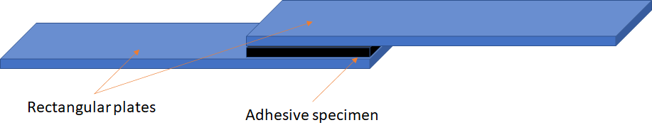
Figure 1. Lap joint shear test.
The plates are pulled apart horizontally until the specimen ruptures and the force-displacement curve is recorded. In this blog post, we analyze an adhesive specimen.
Adhesive Properties
The experimental data used as an example in this blog post is courtesy of Lindhe Xtend AB and gratefully acknowledged. Lindhe Xtend has developed the prosthetic Xtend Foot with its unique lateral flexibility. The lateral flexibility provides unrivaled balance and stability on all surfaces and the user gains increased confidence to move around outdoors and on uneven ground. It reduces the fear of falling, enhances the prospect of moving freely, and increases quality of life for the prosthesis user.
Relevant test data is as follows:
- Thickness of adhesive: 3 mm
- Width of specimen and plates: 25 mm
- Thickness of plates: 5 mm
- Length of adhesive specimen: 5 mm
- Test temperature: 20°C
- Displacement rate: 13 mm/min
The recorded force-displacement curves are shown in Figure 2.
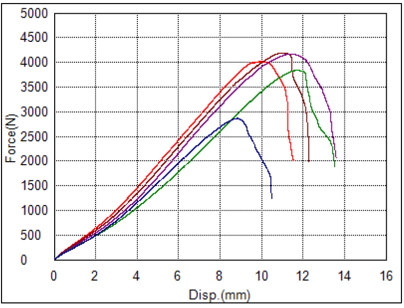
Figure 2. Force-displacement curves for adhesive.
We choose to use the purple curve as a basis for our test. In a stricter analysis, we could determine a mean curve, but for method demonstration, a single curve will suffice. This curve exhibits both initial hardening and subsequent softening due to material rupture. A number of points are chosen to optimize with respect to; see Table 1.
| Displacement [mm] | Force [N] |
|---|---|
| 2 | 577 |
| 4 | 1289 |
| 6 | 2230 |
| 8 | 3224 |
| 10 | 4060 |
| 12 | 4225 |
| 13.5 | 3150 |
Table 1. Selected data points.
Computational Model
Geometric Model
The geometric model is built in the COMSOL Multiphysics® software using the block geometry tools with relevant coordinates; see Figure 3.
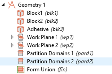
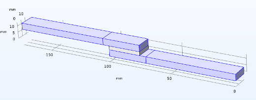
Figure 3. Model geometry.
These blocks are then partitioned to facilitate meshing. Half of the test is modeled, with the symmetry plane along the length of the specimen and plates.
Mesh
The mesh for the optimization scheme is intentionally coarse; see Figure 4.
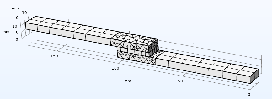
Figure 4. Model mesh.
The exterior plate and adhesive domains are swept, and the plate domains connecting to the adhesive are meshed with free tetrahedrals. The coarse mesh is acceptable, since the result of interest for finding material parameters here is the reaction force. Investigating a detailed stress/strain state in the adhesive would require significant refinement.
Material Model
The plates are much stiffer than the adhesive and could be considered rigid. Here, we assign them material properties of steel (Young’s modulus 210 GPa, Poisson’s ratio 0.3, density 7850 kg/m3). The hyperelastic parameters c_1, c_2, and c_3 for the Yeoh model are all set to 0.1 MPa. In the material model formulation, scaling factors operate on these for an easy optimization scheme. Both material parameters and scaling factors s_{f1yeoh}, s_{f2yeoh}, and s_{f3yeoh} are defined as parameters in COMSOL Multiphysics.
For an easy implementation of our subsequent damage model, we utilize a user-defined strain energy function in the hyperelastic material definition; see Figure 5.

Figure 5. Hyperelastic material definition.
The variable “omeg” modifies the strain energy density, to be explained later. For now, \omega = 1.
Boundary Conditions
Since half of the specimen and plates were modeled, symmetry conditions are applied along the centerplane, as shown in Figure 6.

Figure 6. Symmetry condition (out of plane).
The end face of one specimen is assigned a fixed constraint, and the other end is assigned a prescribed displacement as a function of time, as shown in Figure 7.
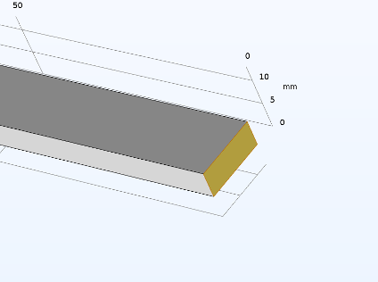

Figure 7. Plate end face boundary conditions. Fixed (left), and prescribed displacement (right).
Study Type and Optimization Setup
Since the damage model to be implemented is based on a rate-form ODE, a time-dependent study is used for the solution. For the hyperelastic model alone, a stationary study would suffice.
Optimizing with respect to our available material data requires us to define the reaction force corresponding to the applied displacement at each time step. To do this, we must enable weak constraints on the prescribed displacement settings and integrate this over the surface, as shown in Figure 8. The factor two is because we are only modeling half of the geometry.
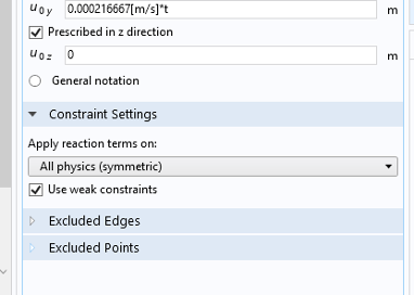
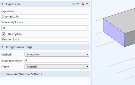
Figure 8. Definition of reaction force for optimization.
Next, we define an Optimization node with a global least-squares objective; see Figure 9.

Figure 9. Optimization setup.
Since we are solving with a time-dependent solver, we must convert the displacements in Table 1 to time in the first column using our defined deformation rate in Figure 7. For our first analysis of a purely hyperelastic model, we only use the first three points, as the subsequent softening requires something more sophisticated.
Finally, we define a time-dependent study and insert an Optimization node; see Figure 10.

Figure 10. Definition of the Optimization node in the study step.
We optimize with respect to the three scaling factors, which operate on the material parameters in the hyperelastic model definition. The only restriction is that s_{f1yeoh} must be nonnegative, as it scales the shear modulus. To keep track of the values of the scaling parameters during solution, it is convenient to define global variable probes of them. This will store them in a probe table for further use.
To define a study with an analysis of the optimized parameters, simply create a new study and set the values of variables solved for to the previous solution, as shown in Figure 11.

Figure 11. Setting up an analysis with the optimized parameter values.
Results: Displacement and Influence of Mesh
The deformation plot is independent of the chosen material parameters, and shown in Figure 12 below, to visualize the state at the end of the analysis.
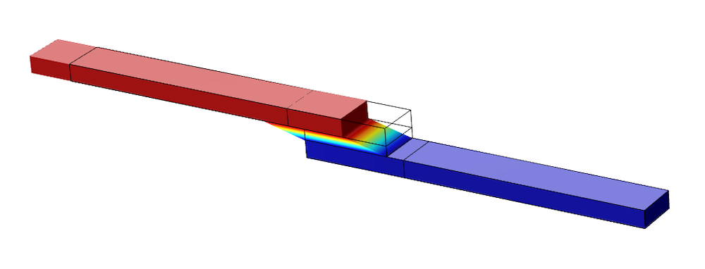
Figure 12. Deformation of the model at the end of the analysis.
As mentioned previously, the mesh will affect the strain state. We also perform an analysis (without damage) of a refined model, shown in Figure 13.
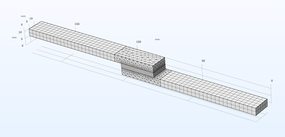
Figure 13. Refined model mesh.
The first principal strain in the adhesive domain at the fourth data point (8 mm) is shown in Figure 14.
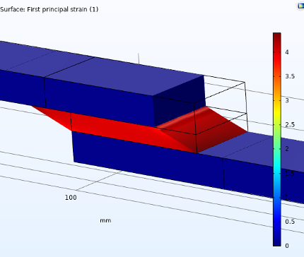
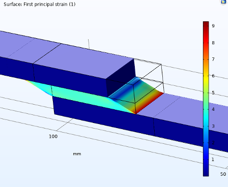
Figure 14. First principal strain in adhesive domain, unrefined (left) and refined (right).
The strain values are far higher in the refined model, and a distinct gradient can be seen that is lacking in the unrefined model. The maximum value of strain over the course of the analysis is shown in Figure 15. The reaction force is also included to show that mesh refinement does not influence it.
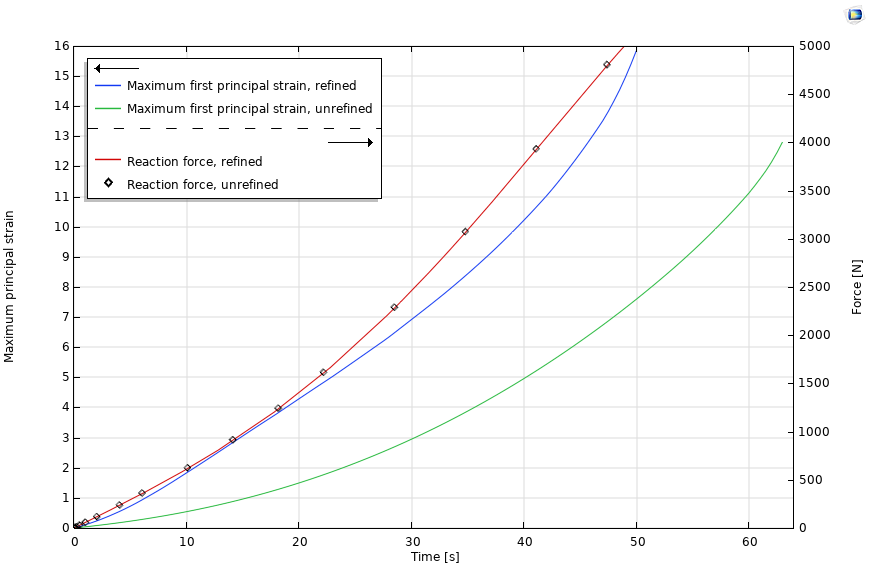
Figure 15. Maximum principal strain and reaction force in adhesive domain. Unrefined and refined mesh results.
Results: Optimized Material Parameters for the Hyperelastic Model
A summary of the material parameters and their optimized counterparts are shown in Table 2.
| Scaling Parameter | Initial Value [-] | Optimized Value [-] |
|---|---|---|
| s_{f1yeoh} | 7 | 6.56 |
| s_{f2yeoh} | 0.09 | 0.34 |
| s_{f3yeoh} | 0.03 | -0.0072 |
| Least squares objective [N2] | ||
| 1.28e-14 |
Table 2. Initial and optimized scaling and material parameters; no damage.
The resulting force-displacement curve is shown in Figure 16.
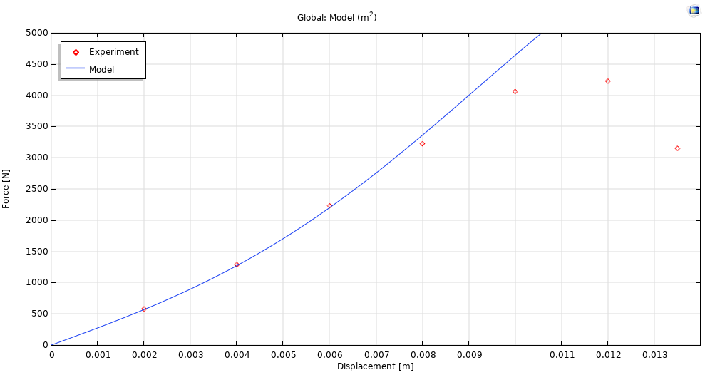
Figure 16. Force-displacement curve for hyperelastic model.
There is excellent agreement between the Yeoh model predictions and experimental data until softening.
Stay Tuned
We will also propose a physically motivated damage evolution law for the material, which is easy to implement and incorporates material softening (monotonic and cycling loading), creep, and stabilization of hysteresis curves during cycling.
Check back for Part 2 of this blog series.
About the Author
Björn Fallqvist is a consultant at Lightness by Design working with product development based on numerical analysis. He obtained a PhD from the Royal Institute of Technology in 2016, working with developing constitutive models to capture the mechanical behavior of biological cells. His main professional interest and specialization is in the fields of material characterization and using various material models to capture physical phenomena.
References
- C. Kumar, “Fitting Measured Data to Different Hyperelastic Material Models“, COMSOL Blog, 2015.
- O.H. Yeoh, “Some forms of the strain energy function for rubber”, Rubber Chemistry and Technology, 5, vol. 66, pp. 754–771, 1993.

Comments (3)
Arijit Garai
April 21, 2022Dear Björn Fallqvist,
I need to solve evolution equation in “Domain ODE and DAE module” in coupling with “Solid mechanics” interface. The evolution contain stretch(solid.UstchZZ) term. Your “Implementing damage evolution” problem has few similarities with mine. I request if you can send me comsol .mph file, then it will be very helpful for me.
Maja Hyldgaard
September 26, 2024Dear Björn Fallqvist
Is it possible to get the files for this paper?
Evan Sisler
December 12, 2024 COMSOL EmployeeHi Maja,
Thank you for your comment! Unfortunately, the model files for this tutorial are unavailable. Please contact our Support team using your COMSOL Access account at https://www.comsol.com/support with any modeling questions.