Wouldn’t it be great if you could include mathematical expressions in plot titles? As of version 6.2 of the COMSOL Multiphysics® software, it’s possible to do so using LaTeX, which is a high-quality, document-preparation system for mathematical and scientific typesetting. In version 6.2, it is also easy to create multiline plot titles. In this blog post, we will explore these new capabilities.
About LaTeX
LaTeX supports visually appealing and comprehensive typesetting of complex mathematical expressions. Previous versions of COMSOL Multiphysics® supported LaTeX segments in reports, and with the extended support introduced in version 6.2, plot titles can now also be enriched with mathematical content.
The LaTeX system contains a large number of elements for creating mathematical expressions, including:
- Greek letters and other special characters, including Unicode characters
- Mathematical symbols and operators
- Delimiters and spaces
- Mathematical function names
- Special mathematical typesetting for fractions and roots
- Text and font elements such as superscript, subscript, overlining, underlining, and italics
The COMSOL Multiphysics Reference Manual includes lists of all the supported LaTeX commands. All of the commands start with a backslash. For example, \alpha is used for the Greek character \alpha.
Adding LaTeX Segments to Plot Titles
It is easy to add mathematical expressions in a plot title using LaTeX. The process is as follows:
- Locate the Title section in the Settings window for a plot group or plot.
- In the title settings, choose Manual from the Title type list.
- In the Title field, add the text with one or more LaTeX segments.
To add LaTeX commands in the Title field, enclose them in either \[ and \] or /$ and /$, invoking one of two LaTeX modes:
- Use
\[and\]around the LaTeX mathematical expression for the display math mode. The display math mode uses more vertical space for the math expression, but it doesn’t add a new line like when using display math mode for standard LaTeX. - Use
/$and/$around the LaTeX mathematical expression for the inline math mode. The inline math mode is meant to be included inline in the text (in standard LaTeX) and has a more compact presentation. The compact presentation may make this mode less suitable for large mathematical expressions.
Conversely, you can convert part of a LaTeX command to be formatted in a different mode type, such as in cases where you want to mix the LaTeX formatting types but don’t want to break up and rewrite the expressions. For instance, to convert a LaTeX command from inline math mode to display math mode, use the special command \displaystyle, and use \textstyle to convert from display math mode to inline math mode.
In the following examples, we’ll take a look at how to add equations and other mathematical expressions to plot titles.
Examples of Math Expressions
Adding Magnetic Field Equations
When plotting the solution of field equations computed using COMSOL Multiphysics®, it can be of interest to include those equations in the plot title. As an example, we’ll use the Submarine Cable 8a — Inductive Effects 3D model from the AC/DC Module Application Library. It uses the Magnetic Fields interface, solving for the magnetic potential A and its components. The solved equations include:
To create a multiline plot title such as this in the COMSOL Desktop®, simply start a new line after each expression (using the Enter or Return key, depending on your keyboard). For this example, enter the title as:
Magnetic field equations:

\[\nabla \times \textbf{H} = \textbf{J}\]

\[\textbf{B} =\nabla \times \textbf{A}\]

\[\textbf{J}  = \sigma\textbf{E} + j\omega\textbf{D} + \textbf{J}_{e}\]

\[\textbf{E} = -j\omega\textbf{A}\]
There are some characteristics to note about this title:
- The
\nablacommand creates a nabla symbol (\nabla). - The
\textbfcommand makes the text appear with a bold font to symbolize a vector quantity. - The
_(underscore) symbol makes the subsequent characters appear in subscript. - The title appears on five lines since four line breaks were entered in the Title field.
- These equations are written in the display math mode, though in this case there isn’t a notable difference between the display and inline math modes.
In the image below, you can see how the expression appears as a title.
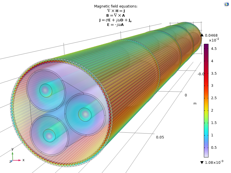
A plot of inductive effects in a submarine cable with the magnetic field equations as the plot title.
Adding Function Limits
A type of mathematical expression that requires some vertical space is the limit expression, which describes the value of a mathematical function as its function argument approaches some limit. Such limits are common in calculus courses and can be formulated like the following example:
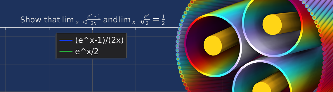
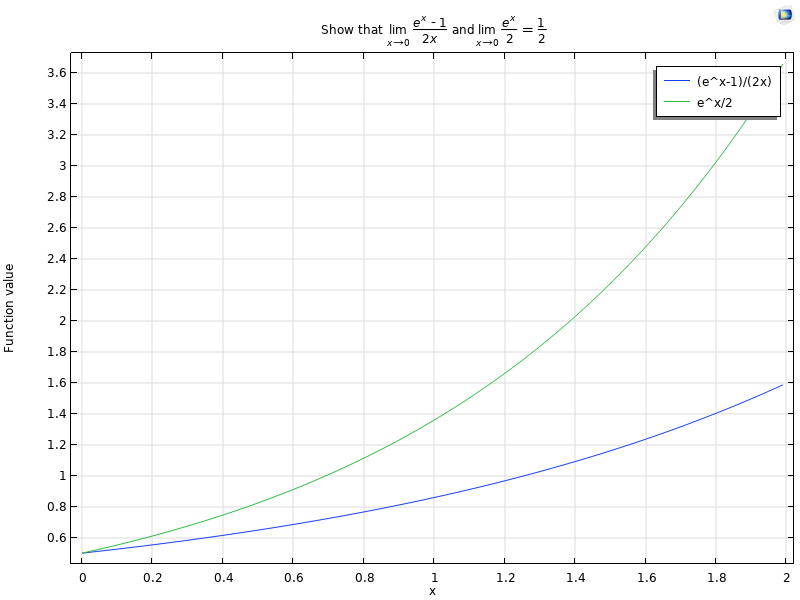
Show that \displaystyle\lim_{x\to 0}{\frac{e^x-1}{2x}} and \displaystyle\lim_{x\to 0}{\frac{e^x}{2}} are equal to 1/2.
The second limit expression is mathematically easy: By inserting 0 for x in the numerator, you get a value of 0.5, as expected. The first limit expression is trickier because inserting 0 for both cases of x results in an undefined 0 divided by 0. Still, when x approaches 0 in the limit, the function value can approach a number that is well defined. In mathematics, you could use l’Hôpital’s rule, which states that the limit of the quotient of two functions is the same as the limit of the quotient of those functions’ derivatives. Using differentiation rules from calculus, you can see that the second limit’s numerator and denominator are the derivatives of the first limit’s numerator and denominator, respectively, which shows that the limit in the first case is also 1/2. In the COMSOL Multiphysics® plot shown below, we have plotted the two functions in an interval that starts with a value close to 0. It seems evident from the plot that both functions approach 0.5 as the function argument approaches 0.
To add the title shown in the image, use the following text:
Show that \[\lim_{x\to 0}{\frac{e^x-1}{2x}} \textrm{ and} \lim_{x\to 0}{\frac{e^x}{2}}={\frac{1}{2}}\]
Here is some notable information about this title:
- Only one math expression segment using the display math mode has been used. To get the “and” to appear as normal text in Roman font, the
\textrmcommand is used. An alternative would be to use two mathematical expressions, with “and” surrounded by spaces between those expressions. - The
\limand\fraccommands in LaTeX create a limit and a fraction, respectively. The\tocommand in the limit’s subscript is a right-pointing arrow. - The limit with subscript x \to 0 takes up some vertical space, so it’s best to use the display math mode with
/[and\]. If you use the inline math mode, the subscript arrow doesn’t fit underneath \lim, as can be seen here:
To make this particular title look good using the inline math mode, you can enclose the \lim_{x\to 0} part using the \displaystyle command to convert it to the display mode: \displaystyle{\lim_{x\to 0}}. It then looks similar to the title in the plot below.
This plot uses a title that shows a mathematical expression with a statement that the plot shows to be correct, as both curves approach 0.5 when x approaches 0.
Concluding Thoughts
In this blog post, we have shown a couple of examples of how you can use LaTeX in plot titles to enhance them with mathematical expressions. We have also discussed how to create multiline plot titles. With all of the LaTeX commands at your disposal, the possibilities to include equations and other mathematical content in plot titles are endless. We hope that these examples can serve as inspiration for plot titles in your own modeling projects.


Comments (0)