
Following up on a previous blog post about glacier flow modeling, we are going to delve a bit further into a crucial component of geophysics modeling in general: parameterizing numerical models using observations. Let’s see how we can quantify sensitivity and infer unknown parameters through indirect observations using the COMSOL Multiphysics® software and add-on Optimization Module.
Coupling Models and Data
A model always requires the knowledge of input parameters, sometimes lots of them. While some of these parameters are well known and easy to find (the density of water or the ideal gas constant, for example), there are often parameters that, for various reasons, are unknown. In the example of glaciology, one difficulty is that ice is generally hard to reach (high altitudes and extreme latitudes), and temperatures and weather conditions make field work challenging. Also, polar caps and mountain glaciers present very wide surfaces to cover.
The method in these cases consists of using indirect observations and modeling to infer the quantity we want to find. In glaciology, surface topography and surface velocity are the greatest sources of data thanks to satellites and radar interferometry (InSAR). On the contrary, basal slipperiness and bedrock topography are hard to access and measure.
In that situation, optimization provides capabilities to use real observations of the state of a system in order to infer the value of the input parameter. This is called inverse modeling, since we deduce values of input parameters from observations of the solution (output). To do so, we minimize a function called an objective or cost function, which quantifies how far the computed solution is from observations. Assuming a solution u and observations of this solution u_{obs}, the cost function j is written j=\|u-u_{obs}\|, thus we adjust the parameters that are unknown (or poorly known) so that u gets closer to u_{obs} and j gets smaller.
The classic way to perform inverse modeling is through a trial-and-error approach, but for vector-valued parameters, this could get extremely tedious. A more systematic approach is to compute the gradient of the cost function j with respect to the parameters and to use that information to determine if every value of our parameters should increase or decrease. This is known as gradient-based optimization.
Computing the Gradient with COMSOL Multiphysics®
Consider a problem, M, which involves a collection of m parameters \alpha whose solution is an n-component vector u, such that M(u(\alpha))=0. First, we define a cost function j(u(\alpha)), which we want to minimize by finding \partial j/\partial \alpha_k for each of the parameters \alpha_k, 1\leq k \leq m. The chain rule tells us:
The cost function is explicitly known, but we still need to calculate \frac{\partial u}{\partial \alpha_k}. Again, using the chain formula, we obtain:
where the n-by-n matrix \frac{\partial M}{\partial u} is the Jacobian of our problem.
At this point, the immediate solution is to solve the n-by-n linear system for the m parameters. However, this forward approach is computationally expensive, since m counts all of the control variables with their discretization. For instance, a global scalar control variable costs one solution and a spatially distributed control variable costs at least N solutions with N mesh elements (assuming it is discretized at order 0, which is constant by element).
The preferred solution is the adjoint approach, the default in the COMSOL® software. Rewriting the previous formula, we find that:
Let’s introduce the adjoint solution vector u^* , defined by:
Multiplying from the right by the system Jacobian \frac{\partial M}{\partial u} and transposing leads to a single n-by-n linear system:
Once this system is solved and u^* is known, the computation of the m components of the gradient is reduced to m matrix-vector product.
This approach, less easily derived in infinite dimension, is based on duality theory and optimal control. Details can be found in J.L. Lions, Optimal Control of Systems Governed by Partial Differential Equations, Springer-Verlag, 1971.
Analyzing a Glacier via Gradient-Based Optimization
The 2D model discussed here can be seen as the central flowline of an actual glacier, but the results can be extended to 3D. The geometry is inspired by the Haut glacier d’Arolla in the Swiss Alps, which is 5 kilometers long and up to 200 meters thick with an average slope of 15%.
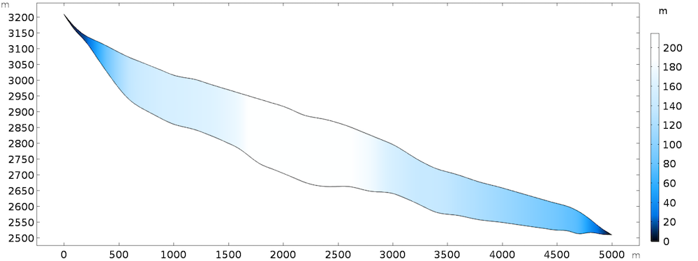
Model geometry, colored by thickness.
The boundary conditions include basal slip at the lower boundary and open boundary at the surface. The constitutive law for the fluid is a non-Newtonian power law with temperature dependency. The sliding at the base is given by a viscous Navier slip with a varying slip length:
\begin{cases}
20m \mbox{ if } 0\leq x \leq 1000 \\
50m \mbox{ if } 1000\leq x \leq 4000 \\
200m \mbox{ if } 4000\leq x \leq 5000
\end{cases}
We impose this varying slip length to make it more challenging when trying to infer it from observations. All of the details can be found in the previous blog post on modeling ice flow. The temperature is imposed at -20°C at the surface and -5°C at the base.
The steady-state solution returns the following velocity field:
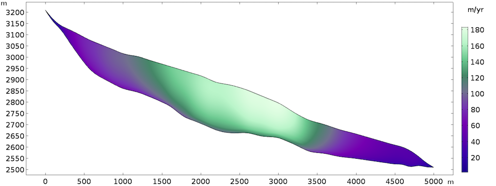
Computed velocity field.
A classical method to build tests and examples without data is the twin experiment method. You simply solve a problem with a given set of parameters and extract the solution values that will serve as data. We can change the values of the parameters and perform data assimilation to infer the original values used to generate the data. To perform a realistic twin experiment, it is important to add some Gaussian (white) noise to the data extracted from the numerical solution. If not, we would commit what is sometimes referred to as the inverse crime.
Performing a Sensitivity Analysis
The first stage of our inverse analysis is sensitivity. For this step, we assume that the geometry is accurately known and focus on surface velocity data. To manufacture our data, we simply use the Export node in the Results section to export, on a subset of data restricted to the surface, the tangential velocity with some added uniform noise (using a predefined random function). Here, we add 10% noise mimicking a typical measurement error.

Left: Data Export node. Right: Original surface velocities and manufactured data.
Let’s compute the sensitivities (gradients) of the model with respect to several control variables. As the cost of computing the gradient is identical regardless of the number of control variables, we compute the gradients with respect to the slip length L_s (defined on the bottom boundary); the viscosity \mu; and the density \rho, defined on the whole bulk.
Next, we add a Sensitivity node and define as many control variable fields as necessary. For each control variable field, we define the control variable name; the initial value (which, in terms of gradient, is the point of linearization); and the discretization. In the present example, we discretize every control variable with discontinuous constant Lagrange functions so that the variables are constant by element/edge, making the simulation faster to solve and easier to scale.

Illustration of the definition of a control variable field for the slip length.
The control variable name defined in the Sensitivity interface must be the one used inside the physics settings in order for it to be taken into account.
Then, we need to define the cost function based on our surface velocity observations. A classical least-square approach lets us define the cost function as the L^2 norm on the surface \Gamma_s of the difference between computed and observed tangential surface velocities:
where u_{obs} is defined using an interpolation function of the exported data file.
The definition of the cost function in the Sensitivity interface uses the Integral Objective node. In the present case, the integration is chosen on the surface \Gamma_s.

Finally, we add a Sensitivity step in the study, which allows us to choose one or more cost functions and control variables among what are defined in the Sensitivity node. The study also defines the gradient method (Adjoint by default).
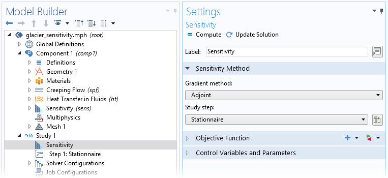
In this case, we don’t need to modify the Sensitivity study step, since the settings are already defined in the Sensitivity node. We can simply run the study.
The study computes the solution for the values of the control variables given in the Sensitivity node as initial values (different from the “real” values used to generate the data). Then, we transpose the Jacobian of the direct problem to solve the adjoint problem to finally compute sensitivities.
Recall that the sensitivities are the gradient of the cost function with respect to the control variables, and they have the same dimension as their corresponding variable. A major consequence of the discretization is that for vector-valued control variables (i.e., any control variable but the global scalar ones), each component of the gradient is scaled by the local size of the mesh elements. This is normal in optimization, but prevents a readable sensitivity map on anisotropic meshes. In particular, control variables discretized using a constant discontinuous shape function need to be normalized by the mesh edge length h_k on which they are defined (i.e., the area of the element for a control variable defined in the bulk or the length of the edge for a control variable defined on a boundary).
Also note that gradient values depend on the absolute values of the original parameters and cost function. To compare the two values, they need to be scaled. For a control variable component \alpha_k and a sensitivity \widetilde{\alpha_k}=\partial j/\partial \alpha_k, the scaled and mesh-normalized sensitivity \widetilde{\alpha_k}^* is written:
where h is the element size directly given by variable dvol, \alpha_0 is the value of the control variable given as the initial value, and j(\alpha_0) is the actual value of the cost function (typically given by variable opt.iobj1). The absolute value is taken because the sign of the gradient is not really relevant for a sensitivity assessment.
That being said, we can now look at our scaled sensitivities. First are the sensitivities with respect to viscosity and density.
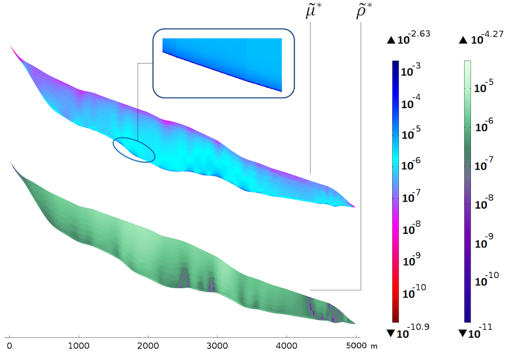
Sensitivities with respect to the viscosity (top) and density (bottom). The color table is logarithmic.
The bottom plot of \widetilde{\rho}^* shows that the sensitivity is rather uniform with the thickness, yet a bit higher approaching the surface. The homogeneous distribution with the thickness seems natural, since the density mainly appears in the gravity terms through the hydrostatic pressure, which is linear with depth. There is a correlation between the slope changes in the bedrock and “columns” of higher sensitivity. The fact that the sensitivity is higher close to the surface could be because of the surface velocities: A deviation from the real density is a bit more noticeable close to the data points.
The top plot of \widetilde{\mu}^* shows a very different picture. The sensitivity clearly increases with depth and a thin layer of very high sensitivity appears along the bedrock. This is explained by the dependency of the sliding boundary condition to the viscosity. For compared values, the maximum for \widetilde{\mu}^* is around 50 times that of \widetilde{\rho}^*, so the model is clearly more sensitive to a perturbation in the viscosity than the density.
Take a closer look at the bedrock sensitivity in the plot below, which shows the scaled sensitivity with respect to the slip length \widetilde{L_s}^*. As a comparison, we also plot \widetilde{\mu}^* along the bedrock.
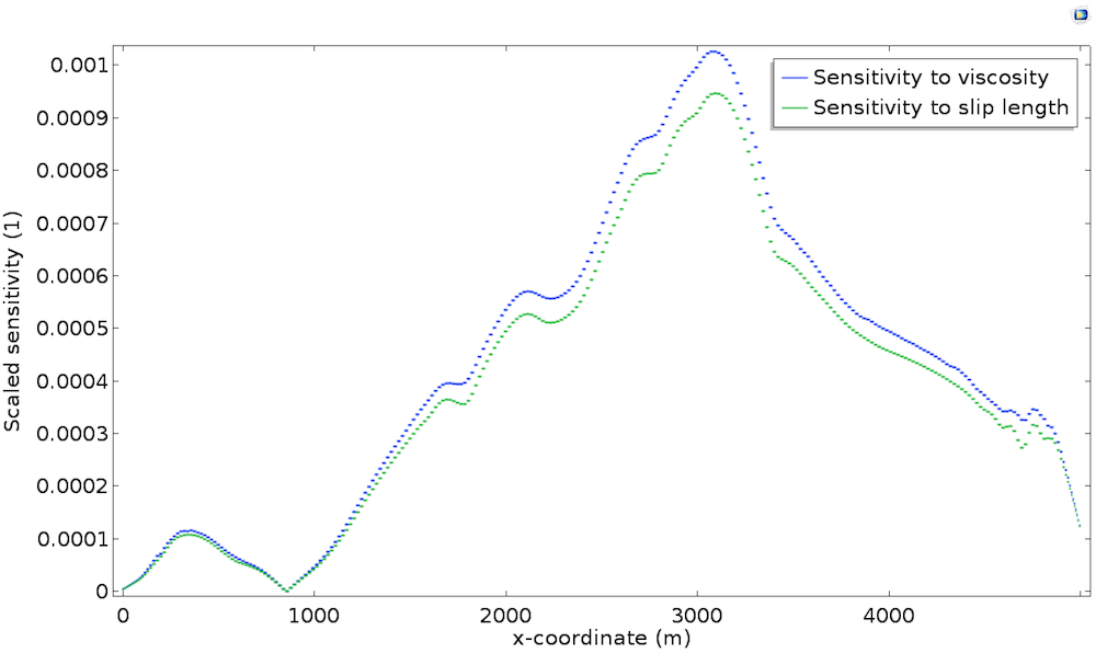
We can see that both sensitivities are strongly correlated with topography and thickness, but mostly, we observe that both sensitivities are almost identical. This is explained by the fact that, at the bedrock, viscosity \mu and slip length L_s play the same role. Indeed, as described in the previous post, the Navier Slip boundary condition is written u_t=\frac{L_s}{\mu}\tau_{nt} so that the sliding is proportional to \mu/L_s. Thus, perturbation in the viscosity is identical to a perturbation in the slip length in terms of model response.
We retain two essential points about the highest sensitivities, which:
- Appear on the slip length and the viscosity, and are localized on the bedrock
- Are strongly correlated with the topography of the bedrock (making them both crucial and poorly observed)
Since viscosity and slip length play the same role in basal sliding, it is clear that data assimilation efforts must focus on the least accurately measured quantity, which is the slip length. Rigorous lab work has been done to derive the constitutive law for viscosity, whereas measurements of slip length are mostly unavailable.
Data Assimilation
Let’s move on to actual parameter identification tests. Based on the previous conclusions, we perform two experiments to identify:
- Slip length along the bedrock
- Shape of the bedrock
For the identification of the slip length, we just need to replace the sensitivity study with an optimization study. The nodes aren’t really different. A slightly more convenient option is available in the Optimization node to define the cost function: the Least-Squares Objective node, which saves us from defining an interpolation function and writing the least-squares cost function. Instead, we can point directly to the data file.

We then need to specify its structure using the subnodes Coordinate column and Value column.
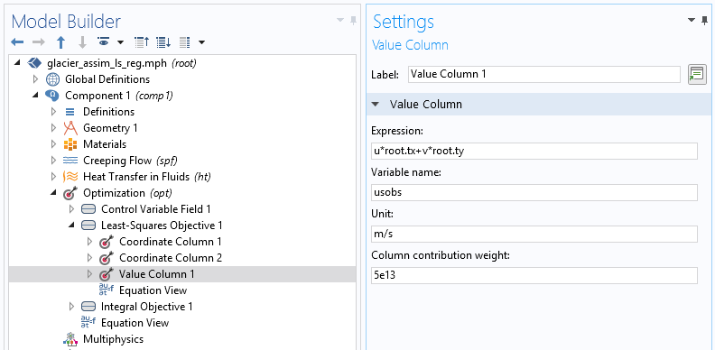
In the two-coordinate column, the first column contains x-coordinates and the second contains y-coordinates for the data point. The Value column is used to find, in terms of model variables, the quantity provided by the data file (tangential velocity). The unit is important for precision (in case, for example, the data file contains velocity in meters per year). The weight is also important for the optimization algorithm. Since the least-squares cost function is not normalized, this value is essential to scale what is considered to be a minimization of the objective. The function is completely model dependent and generally requires a few tries to be correctly adjusted.
With a default value of 1 and a very small absolute value of the cost function (since it’s a velocity), the optimization algorithm exits immediately with the message:
If possible, to help the optimization algorithm, we can define bounds for the control variables based on physical considerations to restrain the acceptable space of minimization. The bounds can be directly defined in the Optimization node as a subnode of the control variable definition.
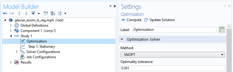
We also need to add an Optimization node in the study. We don’t need to tune this Optimization node much, since the information is provided through the Optimization interface. However, the choice of optimization algorithm is important. The default option (Nelder-Mead) is not suited here, since it is a gradient-free solver limited to scalar-valued control variables. We will use the SNOPT solver, which is a very efficient and versatile gradient-based algorithm.
The study converges in 50 iterations and 1 minute. We plot the value of the inferred slip length and the original (target) value:
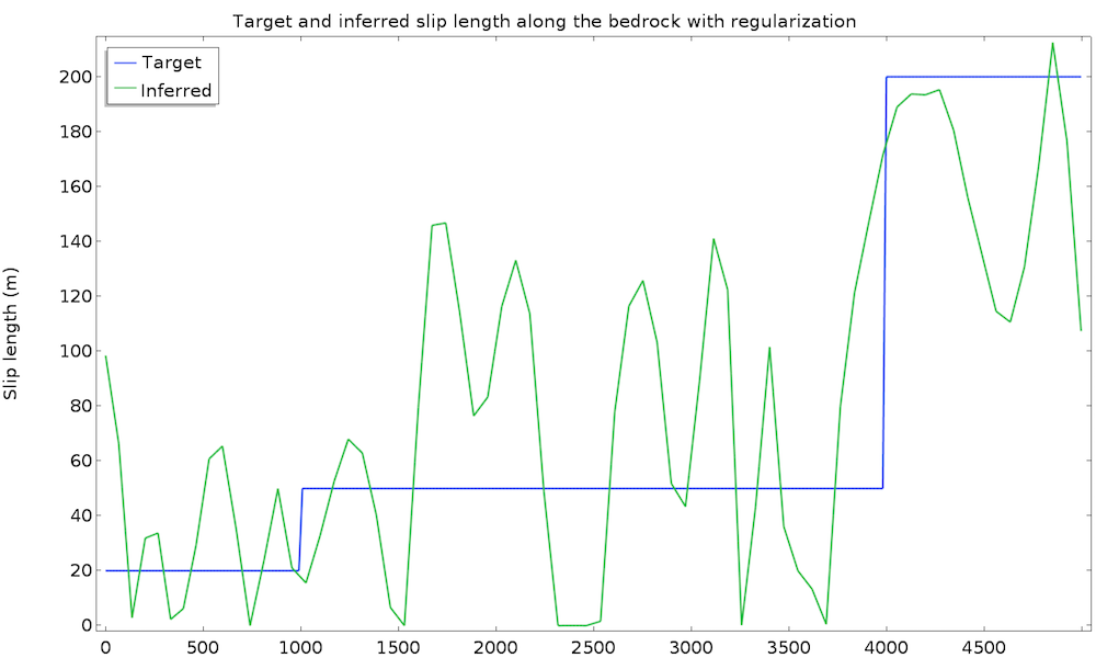
This is a good first result, considering that we guessed the slip length value. However, we can expect a closer value to the real slip length. To improve the identified value, we can introduce some extra information about the slip length. For instance, we can assume a higher regularity of the slip length, since such a quickly varying result does not seem physically appropriate. This idea is called regularization and is almost always used in data assimilation to filter high frequencies in order to more closely retrieve the main component. Regularization is achieved by simply adding a term in the cost function that penalizes over-the-top gradients of our control variable, so minimizing the cost function will require a more regular slip length. We add an Integral objective node defined on the bedrock by \int_{\Gamma_s} \|\nabla L_s\|^2 dx:
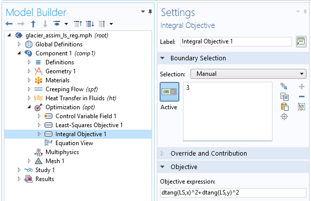
Definition of the extra regularization term.
We run the study again and get convergence in 25 iterations and 30 seconds. The cost function is now made of two terms and the global objective is defined only by the weighted sum of both objectives for the following result:
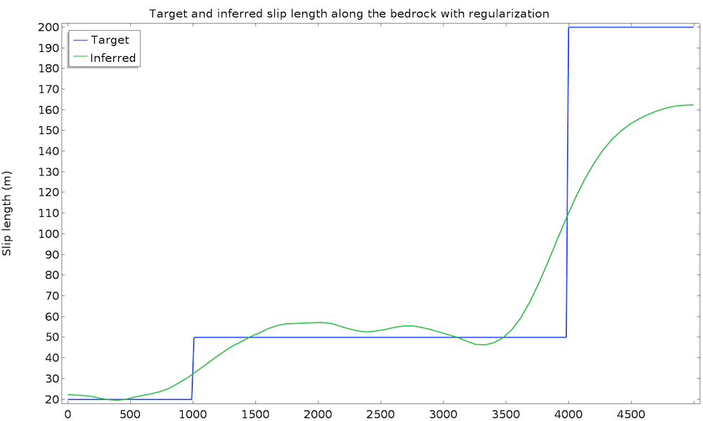
This time, the identified slip length is extremely satisfying and very close to the real value. Remember that we used only 50 data points at the surface with a 10% accuracy, as well as a non-Newtonian, nonisothermal fluid flow model.
Note that no weight has been added to the regularization term because the natural value happened to be well suited. However, the weight generally needs to be adjusted identically to the least-squares term. A regularization that is too large results in a constant identified variable and one that is too small is ineffective.
Now, let’s infer the shape of the topography itself. This example is slightly more complicated, but involves the same process. We want to define a control variable that determines the shape of the bedrock, so we need to find a way to deform the bottom boundary. We could define a displacement d_b on the boundary and a homothetic vertical stretch factor, such that the deformation is maximum at the boundary and decreases with thickness to reach zero at the surface. Given that y_b(x) is the height of the bottom boundary and y_s(x) is the height of the surface, this factor is simply given by (y-y_s)/(y_b-y_s) and the deformation of the domain is written:
where d_c is the control variable defined on the bedrock.
This deformation is introduced using an ALE moving mesh functionality. The cost function remains the same and regularization on d_c is also introduced. To simplify, we run the identification on the same example as before but assume zero velocity at the bedrock for synthetic data. This is because when the slip length is high, the role of the topography is strongly diminished and it can get harder to accurately identify it. With a no-slip condition at the bottom, the geometry makes the value easier to retrieve.
The results show the evolution of the shape of the domain during the optimization process from the initial geometry to convergence. In the animation below, the green background represents the target geometry and the black grid is the optimized mesh. The results achieve really good precision. Neither end of the geometry is very well adjusted, but this is natural, since the velocity goes to zero and so do the cost function and gradient.
Concluding Remarks
Inverse modeling is a very powerful tool. It requires some knowledge of optimization to define a relevant cost function (with possible regularization) and some physical insights to discriminate between control variables. Sensitivity analysis is a good place to start for additional insight into how perturbation on an inlet parameter propagates through a model and impacts a solution.
In general, you should infer as few parameters as possible (ideally one) at a time, because identifying several parameters at once generally leads to what is called equifinality. This is when different sets of parameters lead to similar solutions. Considering that our data is limited in precision, the solutions could be indistinguishable, with the problem growing as the parameters increase.
Next Step
Learn more about how optimization can improve your modeling outcomes by contacting us.


Comments (7)
mohammad albusairi
July 20, 2018It was beneficial Nathan thank you. I’m wondering if its possible to determine the sensitivity wrt a spatially varying control variable (k is a space index) using the sensitivity module.
mohammad albusairi
July 20, 2018* of a vector-valued objective function.
Sebastien KAWKA
August 13, 2018 COMSOL EmployeeDear Mohammad,
Using the Sensitivity interface, you can define a control variable field distributed over any subset of the geometry.
Best regards,
Michael McCullough
May 17, 2019Hi Nathan,
Thank your kind and constructive descriptions. Is there a way to reach this comsol model file? Thanks!
MM
忠民 朱
August 8, 2019wow ,it helps a lot, could you send the mph file to me ? my email is 591149254@qq.com
Bill shang
October 18, 2019Dear Nathan,
Thank you! Very kind and constructive description! I am a student and I am very interesting in this. Is there a way to get this comsol model file? Thanks a lot! My email address is ‘shenbiao17@mails.ucas.ac.cn’. Hoping for your reply!
Bill
Chiemela Victor Amaechi
November 26, 2019Hi, nice post. Can you send me the mph file to my email? My email is c.amaechi@lancaster.ac.uk