
In this blog post, we work through the three-phase induction motor described in Testing Electromagnetic Analysis Methods (TEAM) workshop problem 30a. We analyze the induction motor in 2D using the transient solver in the Rotating Machinery, Magnetic interface. We investigate the motor’s start-up dynamics by coupling the electromagnetic analysis with the rotor dynamics, including the inertial effects. At the end, we compare the benchmark model’s results with those from the COMSOL Multiphysics simulation.
Constructing an Induction Motor with Simulation
A three-phase induction motor consists of two major parts, the stationary part called a stator and the rotating part called a rotor. The stator consists of laminated stator steel and three-phase coils, while the rotor consists of conductive aluminum and steel. The three-phase exposed winding, labeled A, B, and C in the image below, in the stator lag each other in phase by 120°. Each winding phase spans 45°, with air gaps separating them, and the stator’s outer diameter is 5.7 cm.
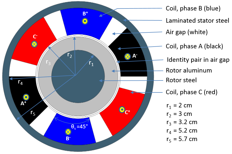
Three-phase induction motor construction depicting the dimensions and phase configurations.
The current density is maintained at 310 A/cm2. This is equivalent to an RMS current of Irms = 2045.175 per winding. The three-phase winding is excited at 60 Hz. Both the rotor and stator steel have a constant relative permeability of μr = 30. The stator steel is laminated and has an electrical conductivity of σ = 0; the rotor steel has an electrical conductivity of σ = 1.6e6 S/m. Similarly, the rotor aluminum has an electrical conductivity σ = 3.72e7 S/m.
Modeling Induction Motor Dynamics in COMSOL Multiphysics
When we construct the geometry of the induction motor in COMSOL Multiphysics, we create two unions. One is for the stator domains and the other is for the rotor domains. We finalize the geometry using the Form Assembly operation, explained in this video, so that the identity pair is automatically between the rotor and the stator.
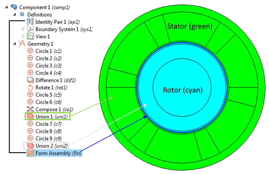
Geometry sequence for an induction motor. The geometry is finalized using Form Assembly between the two unions of rotor and stator.
The material properties used in this model are listed in the following table. The density of the material is not given in the original TEAM document, therefore, we assume the density of the rotor steel and aluminum to be 7850 kg/m3 and 2700 kg/m3, respectively, to compute the rotor inertia.
| Material | Electrical conductivity (σ) | Relative permeability (μr) | Density (ρ) |
|---|---|---|---|
| Rotor steel | 1.6e6 [S/m] | 30 | 7850 [kg/m^3] |
| Stator steel | 0 [S/m] | 30 | Not needed |
| Rotor aluminum | 3.72e7 [S/m] | 1 | 2700 [kg/m^3] |
| Air | 0 [S/m] | 1 | Not needed |
We use the Rotating Machinery, Magnetic interface to simulate the electromagnetic fields in this three-phase induction motor. Since all of the electrical and magnetic material properties are linear, the default Ampère’s Law node works without any modification.
We model the three phases using the Homogenized and Multi-turn Coil features. The number of turns for each winding is n0 = 2045. Each stranded wire carries 1[A] current with 120° out of phase between the three phases. The currents through the three phases are described as:
I A = 1[A]*cos(w0*t)*sqrt(2)I B = 1[A]*cos(w0*t+120[deg])*sqrt(2)I C = 1[A]*cos(w0*t-120[deg])*sqrt(2)
Here, 1[A] is the RMS value of the input current so we need to multiply it with sqrt(2) to make it a peak value.
We can obtain the electromagnetic torque in the rotor directly by using the Force Calculation feature in the Rotating Machinery, Magnetic interface. By adding this feature, the spatial component of the magnetic forces (rmm.Forcex_0, rmm.Forcey_0, rmm.Forcez_0) and the axial torque ( rmm.Tax_0) in this interface can be obtained when postprocessing. The Force Calculation feature simply integrates the Maxwell stresses over the entire outer boundary of the domain selection. Since this method is based on surface integration, the computed force is sensitive to mesh size. When using this method, it is important to always perform a mesh refinement study to correctly compute the force or torque.
The alternative approach would be to use Arkkio’s method of torque calculation, a volume integration of the product of the magnetic flux densities. In this method, the electromagnetic torque in 2D models of electrical rotating machines can be calculated using the following expression:
where r_o is the outer radius, r_i is the inner radius, and S_{ag} is the cross-sectional area of the air gap. The magnetic flux density in the radial and azimuthal directions is B_r and B_\phi, respectively. Refer to the following screenshots for more details on implementing Arkkio’s method in COMSOL Multiphysics.
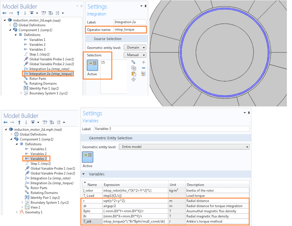
Implementation of Arkkio’s method of torque calculation for an induction motor.
Simulating Motor Dynamics Using the Global ODEs and DAEs interface
The rotational motion of the rotor is given by the following two equations:
(1)
(2)
where T_m is the rotor axial electromagnetic torque, T_L is the load torque, \omega_m is the angular speed of the rotor, and \phi is the angular position of the rotor.
It is modeled using the Global ODE and DAEs interface in two separate Global Equations nodes as shown in the picture below.
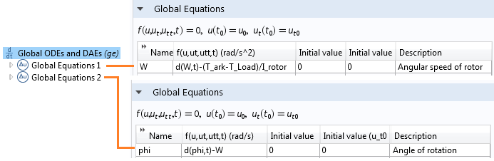
Implementing the differential equations for rotor angular velocity and angle using the Global ODEs and DAEs interface.
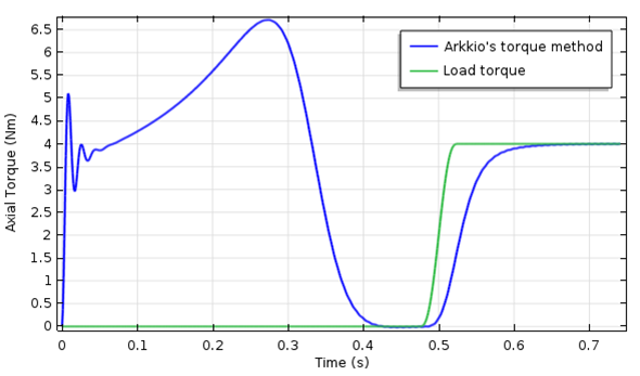
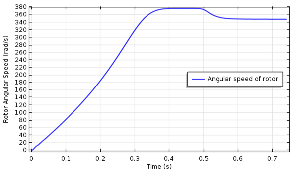
The transient electromagnetic torque on the rotor vs. time (left). The rotor angular speed vs. time (right).
The electromagnetic torque exhibits an oscillatory behavior during the start-up and gradually reaches peak value at around 0.28 seconds. It decreases to zero when it reaches full synchronous speed at around 0.4 seconds. At 0.5 seconds, a step change in the load torque is applied. The motor gradually generates the equal amount of torque by sacrificing some speed.
Comparing the Results from COMSOL Multiphysics and TEAM Problem 30a
To compare the electromagnetic torque, induced voltage, and rotor loss to the results in TEAM problem 30a, we set up the same induction motor model in the frequency domain using the Magnetic Fields physics interface. The rotational motion in this case is introduced using the Lorentz term, which describes velocity. You can download the three-phase induction motor model example here.
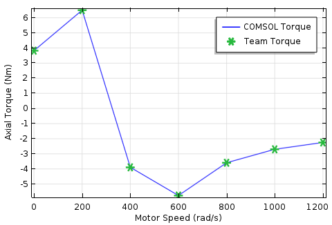
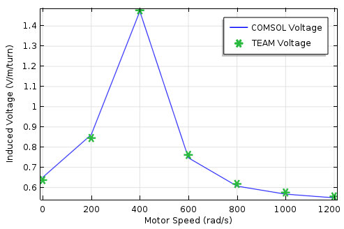
Comparison of axial torque vs. motor speed (left) and induced voltage vs. motor speed (right).
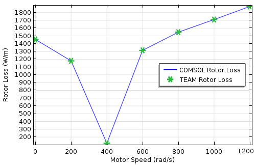
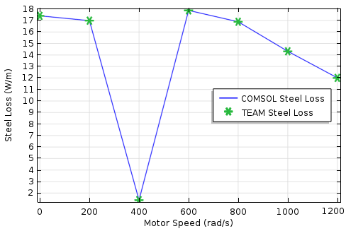
Comparison of rotor loss vs. motor speed (left) and steel loss vs. motor speed (right).
Additional Resources for Modeling Motors in COMSOL Multiphysics
- Try modeling an induction motor by checking out the following tutorial models:
- Learn more about modeling rotating machines in these blog posts:
- Read more blog posts in our Electromagnetic Device series


Comments (2)
Mahdi Mhpoor
September 23, 2016first of all I should say tnx to Nirmal…he always help us without expectation.
But all .mph files , were uploaded in Application Gallery as “Induction Motor in 2D” , are built in later version what unfortunatly isn’t compatible with my version 5.2.0.220
Andrés Yenes
November 12, 2024I’m currently working on modeling a classic squirrel-cage induction motor. In other simulation software (e.g., ANSYS), I’ve noticed that the rotor bars are often modeled without explicitly including the short-circuit ring in the 2D plane being simulated. Instead, they use a termination to effectively short-circuit the rotor bars.
Does COMSOL have an example or recommended approach for this type of setup? Specifically:
– Should the short-circuit ring be modeled explicitly in COMSOL, or is there a way to achieve the equivalent effect using boundary conditions or circuit physics?
– Are there best practices for handling this in a 2D simulation?
Any tips or example models would be highly appreciated.
Thanks in advance for your help!