
We often get questions about how to best evaluate various stress quantities in the COMSOL Multiphysics® software, which provides access to many different stress variables and options for presenting results. In this blog post, we will explore these matters in detail. We will focus on how results evaluation works in general before diving into specifics on stress analysis.
Table of Contents
- What Makes Stresses So Special?
- Some Finite Element Basics
- Physical Continuity
- Averaging Between Elements
- Where Are the Results Evaluated?
- How Stresses Are Computed
- A Special Case: Thermal Expansion
- Pointwise States
- Evaluating Maximum Values
- Which Stress Results Should I Plot?
- Concluding Remarks
What Makes Stresses So Special?
In many areas of physics, the main quantity of interest is the field itself and not its gradients. In a heat transfer analysis, for example, the temperature is usually what you are looking for, while the detailed temperature gradients and heat fluxes are secondary concerns. In structural mechanics, however, the local stresses and strains are often more important than the displacements. In most cases, high stresses will be the cause of failure, either statically or through fatigue. Thus, reliable stress evaluations are important.
Some Finite Element Basics
In the finite element method, the geometry is subdivided into small patches called finite elements that make up a mesh. Within each element, there is an assumption about the variation of the field to be solved for. It is approximated by the shape functions. Most commonly, the shape functions are linear or quadratic polynomials as functions of the coordinates. The field may be a scalar or vector field.
All mesh elements are connected to each other at the mesh nodes. By using equilibrium considerations for some flux, it is possible to set up a system of equations for the value of the field at all mesh nodes.
The field being solved for is summarized in the table below for some common cases:
| Physics | Field | Gradient | Flux |
|---|---|---|---|
| Solid mechanics | Displacement (vector) | Strain (tensor) | Stress (tensor) |
| Heat transfer | Temperature (scalar) | Temperature gradient (vector) | Heat flux (vector) |
| Diffusion | Concentration (scalar) | Concentration gradient (vector) | Mass flux (vector) |
| Electrostatics | Electric potential (scalar) | Electric field (vector) | Electric displacement (vector) |
When the equations generated by the finite element approximation are solved, the dependent variable (degree of freedom or DOF) is known at all mesh nodes. The field is continuous over the entire geometry, and the values at any point inside an element are uniquely defined by the values at the element nodes and the assumed interpolation polynomial (i.e., the shape function).
The gradient of a field, however, is in general not continuous between elements. Inside an element, it is determined by the spatial derivatives of the shape functions and the nodal values at the nodes of the individual element. Thus, the gradients are also uniquely defined within each element but not at element borders. The fluxes are then computed as a function of the gradients. For linear cases, this relation is just a multiplication of the gradient by a given material parameter.
Physical Continuity
It is important to realize that, for physical reasons, fluxes are to a large extent continuous. What flows out of one element should flow into the next. It is only the numerical representation that is not continuous. The finite element solution will, however, converge toward the true, continuous solution as the mesh is refined. Unfortunately for those of us in the stress business, the convergence of gradients is slower than that of the field itself.
The continuity properties of gradients and fluxes are, however, not trivial. If there is a boundary between two different materials, only some components of the flux and gradients are continuous.
As a general rule, the flux is continuous in the direction normal to the boundary but not in the tangential direction. For the gradients, the case is the opposite.
In the example below, stationary heat transfer is studied in a rectangle consisting of two squares with different material properties.

Temperature distribution in a rectangle consisting of a steel square and an aluminum square. The temperature is prescribed along all boundaries with the values shown in the figure.
By plotting the temperature gradients and the heat fluxes along the boundary separating the two domains, the continuity properties can be visualized.


Temperature gradients along the boundary between the materials (left) and heat fluxes along the boundary between the materials (right).
As expected, the temperature gradient in the y direction, as well as the flux in the x direction, is the same on both sides of the interface. If we had done the same exercise for solid mechanics, we would have found continuity in two stress components, \sigma_\mathrm{x} and \tau_\mathrm{xy}, as well as in one strain component, \varepsilon_\mathrm{y}. Another way of viewing this is that those components of the flux that would be possible to prescribe on a free boundary must also be continuous on an internal boundary.
Note that most invariants, such as equivalent stresses or norms of fluxes, will have a jump at a material discontinuity, since not all components of the constituent tensor or vector are continuous.
Averaging Between Elements
Since most quantities that we are studying are known to be continuous, it is tempting to average, for example, stresses between elements. This is also the default setting in most cases. Often, it will not only improve the visual impression, but also be closer to the true, converged solution.
You can control if, and how, averaging (or using the results presentation terminology: smoothing) is applied. The key here is the Quality section that is available for most result presentation nodes.
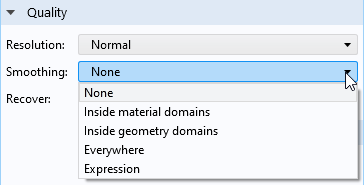
Smoothing options.
The different smoothing options are summarized in the table below:
| Choice | Effect |
|---|---|
| None | No smoothing between adjacent elements. |
| Inside material domains | Smoothing is done between adjacent elements that belong to the same material domain. A material domain is, in it simplest form, a set of domains having the same material assignment. Some physics interfaces do, however, implement their own definitions. One such example is the Shell interface, where elements belong to the same material domain only if they have both the same material and thickness and are not connected by a fold line. Note that this is the default option when you add a new plot. |
| Inside geometry domains | Smoothing is done between adjacent elements that belong to the same geometrical domain but not across domain boundaries. |
| Everywhere | Smoothing is done between all adjacent elements. |
| Expression | Smoothing is performed when a Boolean, user-defined expression evaluates to a nonzero value. |
When smoothing is applied, you can also use a smoothing threshold. This provides a limit for how large the difference in values between adjacent elements at a certain mesh node can be before the smoothing is disabled. The idea is that you should get a compromise where the plots in general are nice and smooth without hiding significant discontinuities.
As of version 6.0 of the COMSOL® software, the default stress plots produced by the structural mechanics interfaces use this functionality. By default, the threshold is set to 0.2, but you can customize this value for your needs.
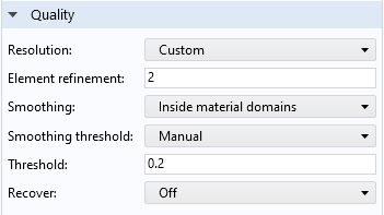
The Quality section of a default plot in the Solid Mechanics interface. With the default threshold value of 0.2, a difference of up to 20% is accepted for smoothing.
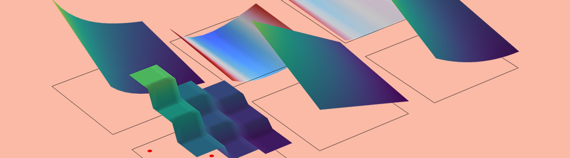
In the figure below, examples of different types of smoothing are shown for a stress plot in a 2D solid mechanics model with a single material. In order to emphasize the effects, first-order triangular elements are used. This is a low-performing element, where the strains and stresses are constant within each element. When looking at the figure, it’s important to note that:
- Without any smoothing (lower-left plot), each element in the mesh is clearly visible.
- When smoothing is performed between all elements (lower-middle plot), the visual impression is much better than without any smoothing. The overall similarity to the “correct” High resolution solution (lower-right plot), which is generated using a fine mesh and quadratic shape functions, is not too bad. However, some details in the highly stressed region are not accurately represented.
- Because only one material is used in this example, there is no difference between the Everywhere (lower-middle plot) and Inside material domains options.
- When the Inside geometry domains option is used (upper-right plot), you can see the stress jumps between the domains, while smoothing is applied within each domain. If different materials had been assigned to the various domains, then a plot with Inside material domains would look similar to this.
- The default settings for structural mechanics are used in the Inside material domains option (upper-left plot). Note that the stress jumps are clearly visible where the stresses are badly resolved, whereas the contours are smooth where the gradients are less pronounced. With this type of plot, you get the best of both worlds: a generally smooth overview, while regions with an insufficient resolution stand out.

The effects of different types of smoothing.
So far, we have been investigating what happens with averaging and jumps in volume, surface, and contour plots. For line graphs, there is an added complexity. If the line has one or more adjacent surfaces, then averaging is needed in two directions:
- Along the line, independently of whether the line is connected to one or more surfaces. This is done in the same way described above, and the same Quality settings section is available.
- Across the line, between adjacent surfaces if there are more than one. This operation is performed first and is unconditional.
If the quantity to be plotted should not be continuous across the line, you no longer want the average value; you want one graph per boundary (3D) or domain (2D). To deal with this situation, you need to use special operators.
If the line represents a boundary in 2D, then you can use the up() and down() operators to specify from which domain the results are taken. The ‘up’ and ‘down’ sides correspond to how the normal vector is oriented on the boundary. This method was used in the abovementioned heat flux graphs. Below is the graph of the temperature gradient in the x direction repeated, but with the default averaged result also included. Clearly, the default averaging is not a good choice when there is a physical discontinuity when crossing the boundary.

Temperature gradient in the x direction, average value, and values from each domain.
The same technique can also be used for surface plots on internal boundaries in 3D, but in this case it is of course only possible to plot the value from one side at a time.
If the selected line is an edge in 3D, things are somewhat more complicated, since there can be an arbitrary number of boundaries sharing that edge. In this case, you need to use the side() operator to pick values from the individual boundaries. The side operator has a syntax like side(12,shell.mises), where the first argument is the number of the boundary. Thus, you first have to figure out the number of the boundary from which you need the result. One quick way of doing this is to create a surface plot of the built-in variable dom and then simply click the intended boundary to see its number.

Finding the number of a boundary using a surface plot.
Another method to find a boundary number is to move to any node in the Model Builder tree that has a boundary selection and then hover with the mouse pointer over the boundary. The boundary number is dynamically displayed in the upper-left corner of the Graphics window.

Finding the boundary number using a boundary selection feature.
Where Are the Results Evaluated?
When generating color plots and line graphs, the expression to be plotted is usually evaluated at several points inside each element, element boundary, or element edge. The number of evaluation points is controlled by the Resolution setting in the Quality section.
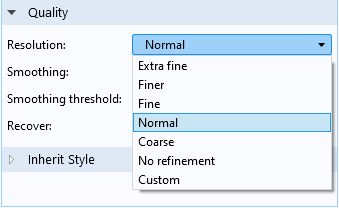
Options for the Resolution.
When one of the predefined resolutions is selected, the number of points that will be evaluated depends on several factors, like model size and space dimension. Using a high resolution will usually generate more detailed plots inside the elements. This is only useful, however, if the evaluated expression actually has a high degree of smoothness inside the element. If not, it will only cause spurious fluctuations.
How Stresses Are Computed
So far, we have mainly covered general result presentation options. When it comes to visualization of stresses, there is one more thing to consider, and that is how the stresses are actually computed within each element.
The total strains are just the derivatives of the displacements, so they are always smooth. The stresses, however, are often the result of a combination of several different effects. The exact details of how stresses are computed depend on the top-level material model and whether geometric nonlinearity is active or not. To explain the general principles, let’s assume that the top level material is linearly elastic and that the analysis is geometrically linear.
Then, the stress tensor, \sigma, is computed as
Here, C is the elasticity tensor, \varepsilon_\mathrm{el} is the elastic strain, and \sigma_\mathrm{add} are any extra stress contributions. The elastic strain is the difference between the total strain \varepsilon_\mathrm{tot}, computed using the shape functions and nodal displacements, and any inelastic strain field \varepsilon_\mathrm{inel}.
Some examples of inelastic strains are:
- Thermal strains
- Hygroscopic swelling strains
- Plastic strains
- Creep strains
- Initial strains
Some examples of extra stress contributions are:
- Viscoelastic stresses
- Stresses caused by damping
- Initial stresses
Thus, the total stress is in general a sum of several different contributions. In particular, \varepsilon_\mathrm{tot} and \varepsilon_\mathrm{inel} are often of the same order of magnitude, so that the elastic strain tensor contains small numbers obtained by the subtraction of two or more large numbers from another. This is the case for unconstrained thermal expansion or large plastic deformations, for example.
So why would this be a problem? If the different stress and strain contributions are not represented by the same type of interpolation over the element, there can be large local fluctuations, even though the results are consistent in an average sense.
A Special Case: Thermal Expansion
Let’s take a short detour to study a common case when this can happen. It was observed early by the finite element community that “wavy” stress patterns can occur in coupled thermal stress analysis. It is most common to use quadratic shape functions for both the displacements and the temperature for coupled thermal stress analysis. Since thermal strains are proportional to the temperature, \varepsilon_\mathrm{inel} will then have a quadratic variation within each element. The total strains, however, are derivatives of the displacement shape functions, and will thus have linear distributions. Now, the elastic strain is computed as the difference between a linear function and a quadratic function. The effect is that there may be a strange elastic strain (and thus stress) pattern inside each element. For this reason, it has sometimes been recommended that the thermal problem be solved using linear shape functions when the temperatures are used to drive thermal expansion in a solid. In COMSOL Multiphysics, this problem is handled internally in the Thermal Expansion multiphysics coupling (and similar features like Hygroscopic Swelling and Intercalation Strain). The inelastic strain field is reinterpolated to a polynomial order that matches the strains computed from the displacement field. This will reduce such artifacts in the local stress solution.
Pointwise States
There is another type of inelastic strain that does not involve fields at all but rather local states stored pointwise at the integration points (Gauss points). For more details about Gauss points, check out our blog post “Introduction to Numerical Integration and Gauss Points”. Most nonlinear material models, like plasticity and creep, work this way. For this case, evaluation of stresses at an arbitrary location in the element becomes more complicated.
If you request a stress component, like solid.sx, it is actually computed “on the fly” at each location in the element. The nonlinear material law is evaluated there, making use of stored values from the closest Gauss point. If the variation of the inelastic strains over the element is large, this can introduce significant errors. There may even be a failure to evaluate the material law, even though it can be evaluated at the Gauss points.
A better approach is to create a smooth approximation based on the Gauss point values. The gpeval() operator provides this possibility. If you, for example, request gpeval(4,solid.sx) rather than solid.sx, you will plot a stress that is smooth over the element. In this case, the nonlinear stress–strain relation is evaluated only at the Gauss points where it is already fulfilled. Then, a least-squares fit of the Gauss point values is used to define a smooth field.
In its raw version, the gpeval() operator requires you to enter the appropriate integration order as the first argument. Fortunately, in most cases you will not have to worry about this. A number of predefined variables are available in the physics interfaces, for example, solid.sGpx and solid.misesGp. If you cannot find a suitable built-in variable for your expression, then you can use a physics interface specific operator, for example, solid.gpeval(expr). The correct integration order is embedded into the operators specific to a physics interface.
In the example below, different evaluation options are explored for a field that has been stored at Gauss points (by a user-defined dependent variable called myDOF). The model consists of a single 2D element, with both the x and y coordinates ranging from 0 to 1. The field is described by the expression (Y+1)/(2*X+1). A 3×3 Gauss point scheme is used, so there will be nine independent numbers stored. These values are exactly those of the original field, evaluated at each Gauss point.

Different type of evaluations of Gauss-point data.
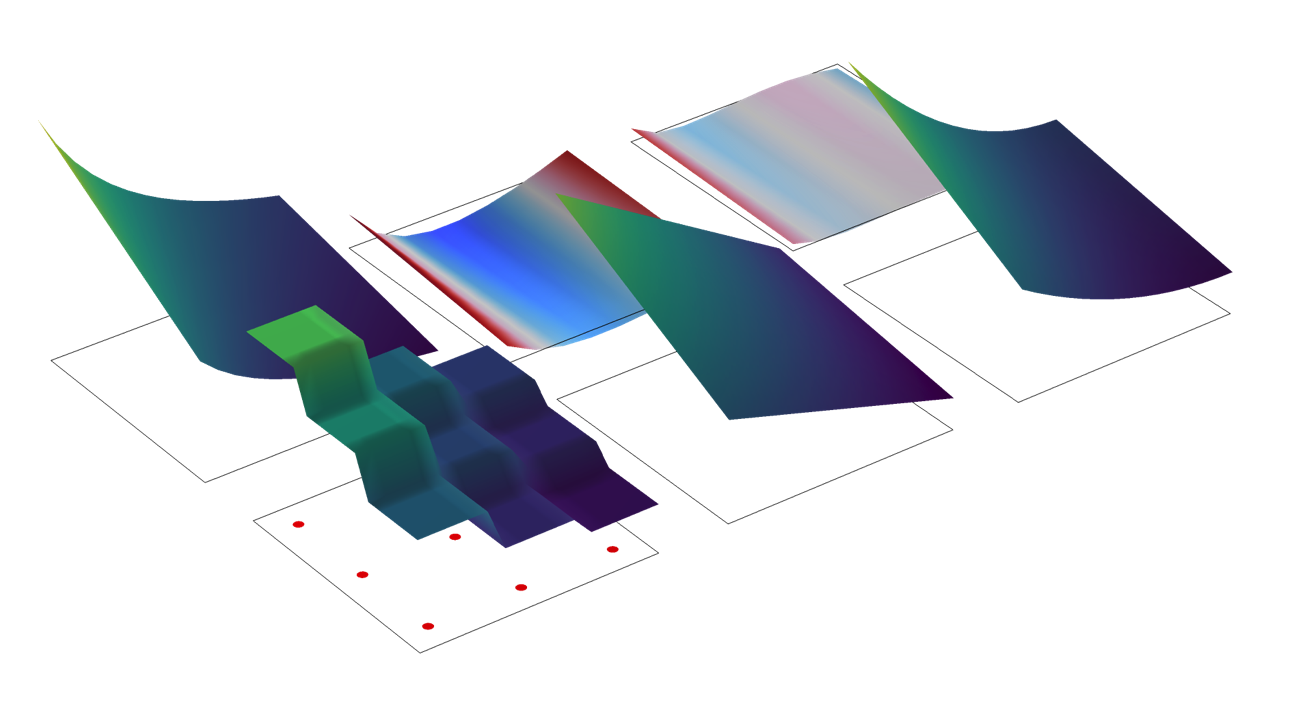
The same data, represented by a height plot.
In the upper-left plot, the original function is visualized. Below it, the behavior of a surface plot of the stored state, myDOF, is shown. In the same plot, the locations of the Gauss points, as well as the stored values, are also indicated. The default behavior, that Gauss point states are represented by the value at the closest Gauss point, is clearly visible. A much better approach in this case is to evaluate a smooth field, using the gpeval() operator. This is shown in the two rightmost plots in the bottom row. The difference between these two plots is the polynomial order of the smoothing field. The default is to use a bilinear field (lower-middle plot). In this example, fitting to a quadratic field is a better option. In the upper-middle and upper-right plots, the difference between the smooth fields and the exact value of the function are shown.
Finally, let’s deal with two common misconceptions:
- If you evaluate an expression like
solid.sxat a Gauss point, you do get the computed value at the Gauss point. However, an expression likesolid.sGpxorgpeval(4,solid.sx)evaluated at a Gauss point will not retrieve the stored result at that point. The reason is that these expressions give smooth fields, obtained by a least-squares fit. A fitted polynomial will not necessarily pass through its data points. - If you evaluate an expression like
gpeval(4,solid.sx)on a boundary, the values at the Gauss points on the boundary are used for setting up the interpolating polynomial. This is probably not what you intend if you are doing a surface plot on the boundary of a solid mechanics model. Fortunately, the built-in quantities likesolid.sGpxandsolid.gpeval(solid.sx)behave as you expect: They use the domain interpolation.
Evaluating Maximum Values
With the toolbox presented above, we can approach the common task of evaluating maximum values. First, it is important to realize that there is no single “correct” method. The only truth would come from performing an analysis with a mesh so fine that the discretization errors were very small. In real life, that is seldom feasible.
With this said, it is usually preferable to use Gauss-point interpolated results, since they are less prone to random fluctuations. However, they may not be best (in the sense of “closest to the truth”) for all cases.
In postprocessing, you can use different approaches for obtaining a maximum value (five of which are shown in the UI image below). You can look at the maximum value on a plot legend (see (1) in the image below) or you can add a:
- Marker subnode to, for example, a volume plot (see (2)).
- The Marker subnode is evaluated using the same data as the plot itself, so the results will always be consistent.
- The evaluation is controlled by the settings in the Quality section of the plot.
- Node like Max/Min Surface to a plot group (see (3)).
- These nodes have their own settings.
- The evaluation is controlled in the Advanced section.
- Node like Surface Maximum under Derived Values (see (4)).
- These nodes have their own settings.
- The evaluation is controlled in the Configuration section.
- Maximum operator under Definitions (see (5)).
- Such operators have their own settings.
- The evaluation is controlled in the Advanced section.
- The operator can be used in a Global Evaluation.
- Graph Marker to a Line Graph.
- The marker is evaluated using the same data as the plot itself, so the results will always be consistent.
- It is controlled by the settings in the Quality section of the plot.
- Point Evaluation node under Derived Values — if the critical point is known.
- A geometrical point will use an averaging from adjacent edges, boundaries, or domains.
- A point from a Cut Point data set will take its value from a single evaluation inside one single element.

Some examples of maximum value evaluations.
It is clear that the values you get using these approaches are not necessarily the same. Some hints:
- If you want to highlight the peak value in a plot or graph, use the corresponding Marker subnode. The viewer of the plot will be confused if the values are not consistent.
- If you want to get a worst case value, use an evaluation that suppresses averaging.
- Surface and volume maximum evaluation may not give the same value, even though the expected maximum is at the surface, as long as smoothing is used or the stress calculation involves pointwise states.
- For structural mechanics problems, maximum stresses often occur at the boundary. If the boundary is not loaded, there is a nice trick to obtain accurate results on it: Add a very thin membrane on top of it, with the same material data as the solid. The membrane acts as a type of virtual strain gauge. In version 6.1, the Thin Layer feature was added to the Solid Mechanics interface. It can be used for the same purpose.
Below is a plot that shows the effects of different options for evaluating the minimum of a stress component, using a marker in surface and volume plots. Both solid.sy and solid.sGpy are plotted with and without averaging. As expected, each value computed without smoothing is higher than the corresponding value with smoothing. It can also be noted that without averaging, surface and volume evaluations give the same result. This is natural, since the peak value is at the surface, so the same peak location is probed in both cases.

The effects of some different evaluation options.
Which Stress Results Should I Plot?
When you select results to plot, you will encounter a menu like the one below:
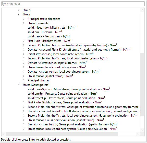
Selecting stress results.
The exact options available will depend on the physics interface and which material models and other options you are using. This may look overwhelming, but there are some quantities that are more important than others.
For isotropic materials, it is most common to use scalar stress measures, like the von Mises or Tresca equivalent stresses. The von Mises stress is popular because it is easily evaluated, and since it is straightforward to compute for example sensitivities. However, the Tresca stress is a better choice if you want to be on the safe side. The value of the Tresca equivalent stress is between 0 and 17% larger than the value of the von Mises stress for a given stress state. In some fields of engineering, like pressure vessels, the Tresca stress is always used, sometimes under the name stress intensity.
Even though the von Mises and Tresca equivalent stresses are quite useful to get an overview of the stress state, they should only be used for evaluating the risk of failure or to find the “most loaded point” for specific classes of materials. These stress measures were originally designed for predicting yielding in metals, and they are insensitive to the mean stress. A metal is no closer to yielding at the bottom of the Mariana Trench than it is in free air! Failure in materials like soils or concrete, on the other hand, is strongly dependent on the mean stress; a state of compression is stabilizing.
Now you may ask: How can I get a plot where the red spot is the critical point if my material is not a metal? The answer contains two parts: First, you cannot in general do that without introducing some material properties describing the failure. Once you have access to those values, you can use the Safety node in the structural mechanics interfaces. In that feature, different types of measures of the margin to failure can be computed for many classes of materials. Since these criteria are often based on the stresses, anything said above about stress evaluation would also apply here.
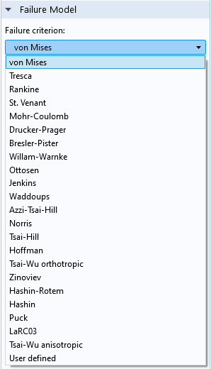
Failure models in the Safety feature.

An analysis of the von Mises stress (above) and safety factor (below) of a soil mechanics problem. The analysis below uses a Drucker–Prager criterion.
Sometimes, you may want to study the individual stress components. This may be because the material is anisotropic or because you want to understand the stress distribution better. In the latter case, it is often useful to plot the principal stresses, too.
When working with individual stress components, it is quite common that you want to evaluate in other directions than the global coordinate system. There are several types of results labeled “local coordinate system”. This means that the orientation is determined by the coordinate system selection in the material node, for example, Linear Elastic Material.
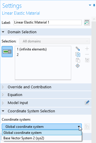
Selecting a coordinate system in a material model.
For an isotropic material, the only effect of the coordinate system selection is to define local directions for results. For anistropic materials, the main purpose of the selection is to provide the reference orientations for the material data. As a side effect, you get stress and strain results in local directions. In version 6.1, a new feature named Local System Results has been added. With this feature, you can assign any local coordinate system to selected domains in order to create variables containing, for example, stress and strain tensors having local orientations.
In COMSOL Multiphysics, there are three types of stress tensors: Cauchy, first Piola–Kirchhoff, and second Piola–Kirchhoff. To learn more about this topic, check out our blog post “Why All These Stresses and Strains?” and our Multiphysics Cyclopedia page on stress and equations of motion. If you plan to study a single component of a stress tensor, the distinctions may be important, but for a geometrically linear analysis, the stress tensors are all identical.
Concluding Remarks
COMSOL Multiphysics provides a multitude of options for fine-tuning the evaluation and presentation of results. To get the most out of your simulation, it is important that you familiarize yourself with these options — what is optimal depends on what you are studying and the purpose of the analysis.
One thing that has not been discussed here is how to deal with high stresses that occur in corners or at other singularities. The effect of singularities is discussed in our blog post “Singularities in Finite Element Models: Dealing with Red Spots”. We will likely come back to this topic of great practical interest.
Next Step
Want to learn more about the software’s stress analysis capabilities? Contact COMSOL by clicking the button below!

Comments (1)
Ivar KJELBERG
May 7, 2022Hei Henrik,
Thanks’ for a detailed BLOG post, as usual a lot of useful facts and details 🙂
Indeed “Solid” as ACDC are true 3D physics requiring to think fully 3D (even for 2D models), and require a careful analysis of the results.
Anticipating your update to the “Red spot stress issues” I may only add that your “filter” plot node is very useful to identify and visualise hot spots (Mises > a_limit), but also the integration of the mesh volume to see total volume (per domain) of these hot spots and to see how they evolve with mesh refinement is nice. Ideally one would need some histogram plots to see how many elements have excessive stress (and for tubular “welded” structures attached together this histogram would be nice if expressed per domain or per tube).
Sincerely,
Ivar